Point Density Surface Set

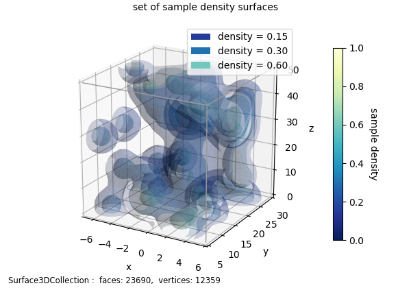
This example illustrates the variation of the cloud density throughout the domain showing a set of constant density surfaces. An array of relative densities are used in the valsurf method. The get_color_for_val method is used to return legend colors for the densities.

import numpy as np
import matplotlib.pyplot as plt
from matplotlib import cm,colors,colormaps,patches
import s3dlib.surface as s3d
import s3dlib.pntcloud as ptc

# 1. Get data to examine ...........................................
npnts,seed,domain = 50, 6, [ [-7,6], [5,30], [0,50] ]
np.random.seed(seed)
xc = np.random.uniform(*domain[0], npnts)
yc = np.random.uniform(*domain[1], npnts)
zc = np.random.uniform(*domain[2], npnts)
input_coor = np.column_stack((xc,yc,zc))

# 2. Setup and map surface .........................................
pdg, drez, relden,cmap = 1.2, 3, 0.3, 'YlGnBu_r'
density_levels = [ .15, .3, .6]

cloudObj = ptc.Point3DCloud(drez,cmap=cmap,domain=domain)
cloudObj.map_vals_from_sampdens(input_coor,pdg)
cloudObj.map_cmap_from_cloudvals()

surface = cloudObj.valsurf( *density_levels )
surface.set_surface_alpha(.2)

# 3. Construct figures, add surfaces, and plot ....................
fig = plt.figure(figsize=(6,4.2))
title='set of sample density surfaces'
fig.text(.5,0.99,title,ha='center',va='top')
fig.text(0.02,0.01,str(surface),ha='left',va='bottom',fontsize='small')
ax = plt.axes(projection='3d', aspect='equal')
ax.set(xlim=domain[0], ylim=domain[1], zlim=domain[2],  
    xlabel='x',ylabel='y',zlabel='z')
ax.view_init(20)
ax.add_collection3d(surface.shade(.1,flat=False).hilite(.5,focus=2,flat=False))
s3d.add_boxCorner(ax,domain)

c,v,n = cloudObj.get_color_for_val(density_levels)
hnd = [ patches.Patch(label='density = {:.2f}'.format(v[i]), facecolor=c[i]) \
    for i in range(len(density_levels)) ]    
ax.legend(handles=hnd)

scmp = cloudObj.cBar_ScalarMappable
cbar = plt.colorbar(scmp, ax=ax,  shrink=0.8, pad=.1 )
cbar.set_label('sample density', rotation=270, labelpad = 15)

fig.tight_layout(pad=2.5)
plt.show()