Bunny Density

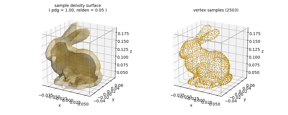
The points are from a Stanford Bunny obj file. Since the method get_surfgeom_from_obj extract the surface directly, the vertices were used as the data samples.

These points define a surface which result in two density surfaces, inner and outer, of constant cloud density.

import numpy as np
import matplotlib.pyplot as plt
import s3dlib.surface as s3d
import s3dlib.pntcloud as ptc

# 1. Get data to examine ...........................................
surface = s3d.get_surfgeom_from_obj("data/bunny.obj")
input_coor = surface.vertices.T
npnts,bounds = len(input_coor) , surface.bounds
domain = [ bounds['xlim'],bounds['ylim'],bounds['zlim'] ]

# 2. Setup and map surface .........................................
pdg, drez, relden = 1.0, 3, 0.05

cloudObj = ptc.Point3DCloud(drez,domain=domain, color='goldenrod')
cloudObj.map_vals_from_sampdens(input_coor,pdg)
surface = cloudObj.valsurf(relden)
surface.set_surface_alpha(.3)
surface.triangulate(1)

# 3. Construct figures, add surfaces, and plot ....................
fig = plt.figure(figsize=(10,4))
# ....................
title = 'sample density surface\n( pdg = {:.2f}, relden = {:.2f} )'.format(pdg,relden)
fig.text(.27,0.9,title,ha='center')
ax = fig.add_subplot(121, projection='3d', aspect='equal')
ax.set(xlim=domain[0], ylim=domain[1], zlim=domain[2],  
    xlabel='x',ylabel='y',zlabel='z')
ax.view_init(20)
ax.add_collection3d(surface.shade(flat=False).hilite(flat=False))
s3d.add_boxCorner(ax,domain)
# ....................
title = 'vertex samples ({})'.format(npnts)
fig.text(.75,0.9,title,ha='center')
ax = fig.add_subplot(122, projection='3d', aspect='equal')
ax.set(xlim=domain[0], ylim=domain[1], zlim=domain[2],  
    xlabel='x',ylabel='y',zlabel='z')
ax.view_init(20)
ax.scatter(*input_coor.T, c='darkgoldenrod', marker='.', s=5)
s3d.add_boxCorner(ax,domain)
# ....................
fig.tight_layout(pad=3)
plt.show()