Unstructured 3-D Coordinate Surface

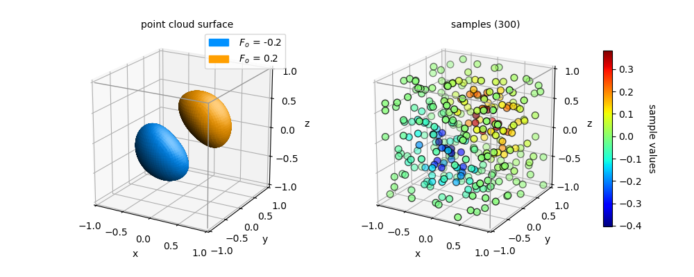
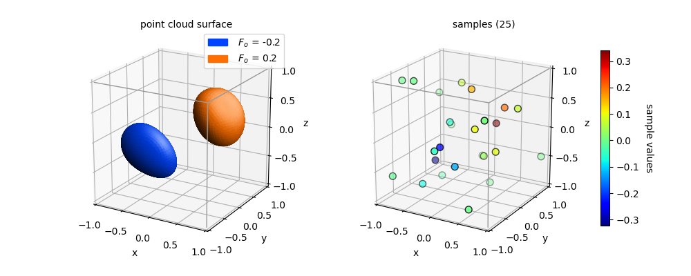
This example uses a distribution of sample values based on the implicit function given in the Contour Surface within a Volume example. Consequentially, the resulting surfaces are similar. With a smaller sample size (N=25), the resulting surface differs from implicit functional surface, as shown below. With a small sample size, the surface difference may be substantial, dependent on the discrepancy of coordinate positions.

import numpy as np
import matplotlib.pyplot as plt
from matplotlib import cm,colors,patches
from scipy.stats.qmc import Halton
import s3dlib.surface as s3d
import s3dlib.pntcloud as ptc

# 1. Get data to examine ...........................................
# 0. control parameters.
drez,N,seed,Fo,cmap = 5, 300, 6, 0.2, 'jet'
domain = [ [-1,1], [-1,1], [-1,1] ]
# generate data points with values .
dt_coor = 2*Halton(3, seed=seed).random(N) - 1
vals = np.sum(dt_coor, axis=1)*np.exp(-3*np.sum(dt_coor**2, axis=1))
points = np.column_stack((dt_coor,vals))

# 2. Setup and map surface .........................................
Fval = [-Fo, Fo]                    #  surface function values.

cloudObj = ptc.Point3DCloud(drez,domain=domain)
cloudObj.map_vals_from_sampvals(points, cmap=cmap)

surface = cloudObj.valsurf(*Fval)
scol,fv,_ = cloudObj.get_color_for_val(Fval)

# 3. Construct figures, add surfaces, and plot ....................
fig = plt.figure(figsize=(10,4))
# ....................
title = 'point cloud surface'
fig.text(.27,0.9,title,ha='center')
ax = fig.add_subplot(121, projection='3d', aspect='equal')
ax.view_init(20,-60)
ax.set(xlim=domain[0], ylim=domain[1], zlim=domain[2],  
    xlabel='x',ylabel='y',zlabel='z')
ax.add_collection3d(surface.shade(ax=ax).hilite(.5,ax=ax))
s3d.add_boxCorner(ax,domain)

hnd = [ patches.Patch(label=r'$\ F_o$ = '+str(fv[0]), color=scol[0] ) ,
        patches.Patch(label=r'$\ F_o$ = '+str(fv[1]), color=scol[1] ) ]
ax.legend(handles=hnd)
# ....................
title = 'samples ({})'.format(N)
fig.text(.7,0.9,title,ha='center')
ax = fig.add_subplot(122, projection='3d', aspect='equal')
ax.view_init(20,-60)
ax.set(xlim=domain[0], ylim=domain[1], zlim=domain[2],  
    xlabel='x',ylabel='y',zlabel='z')
ax.scatter(*dt_coor.T, s=50, c=vals, cmap=cmap ,edgecolor='k')
s3d.add_boxCorner(ax,domain)

norm = colors.Normalize(np.min(vals),np.max(vals) )
cbar =fig.colorbar(cm.ScalarMappable(norm=norm, cmap=cmap), ax=ax,shrink=0.8, pad=.1)
cbar.set_label('sample values', rotation=270, labelpad = 15)
# ....................

fig.tight_layout(pad=3)
plt.show()