Contour Surface within a Volume

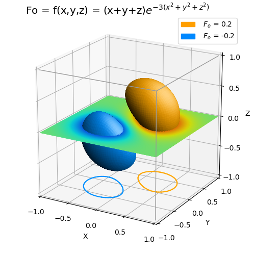
The implsurf method can be used to visualize a ‘contour surface’ (2-D) of constant value for a 3-D volume function, f(x,y,z), within a 3-D domain. The value of the surface is set by the fval argument of the method, which by default is zero. This is analogous to evaluating a ‘contour line’ (1-D) of constant value for a planar function, f(x,y), within a 2-D plane.

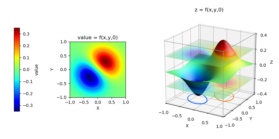
The above figure shows two contour surfaces which are intersected by a plane of constant z=0. The intersection is a contour line in the z-plane. The line contour is also shown below using a planar visualization or by projecting the planar function value in the z-directioon.

import math
import numpy as np
import matplotlib.pyplot as plt
from matplotlib import patches,colormaps
import s3dlib.surface as s3d

# Surface Contours in a Volume

# 1. Define function to examine .....................................
rez, Fo, cmap = 6, 0.2, colormaps['jet']
scol = [ cmap(.26), cmap(.74)]        #  surface colors
dmn = [  [-1,1], [-1,1], [-1,1] ]     #  evaluation domain 

def func3D(xyz) :
    x,y,z = xyz
    f = (x+y+z)*np.exp(-3*(x**2 + y**2 + z**2) )
    return f

# 2. Setup and map surface .........................................

Fvals = [-Fo, Fo]               #  surface function values.
surface = s3d.Surface3DCollection.implsurf( func3D, rez, dmn, *Fvals, cmap=cmap)
surface.evert()

contours = surface.contourLines(1.0e-6).map_to_plane(-1.0)

zplane = s3d.PlanarSurface(rez,'oct1')
zplane.map_cmap_from_op(func3D,cmap)
surface = surface + zplane

# 3. Construct figure, add surface, and plot ......................
ticks = [-1,-.5,0,0.5,1]
info = r"Fo = f(x,y,z) = (x+y+z)$e^{-3(x^2+y^2+z^2)}$ "
fig = plt.figure(figsize=(5,5))
fig.text(0.1,0.99,info, ha='left', va='top', fontsize='x-large')
ax = plt.axes(projection='3d', aspect='equal')
ax.view_init(20,-60)
ax.set(xlim=dmn[0], ylim=dmn[1], zlim=dmn[2],xlabel='X',ylabel='Y',zlabel='Z',
        xticks=ticks, yticks=ticks, zticks=ticks )
hnd = [  patches.Patch(label=r'$\ F_o$ = '+str(Fvals[0]), color=scol[0] ) ,
         patches.Patch(label=r'$\ F_o$ = '+str(Fvals[1]), color=scol[1] ) ]
ax.legend(handles=hnd)

ax.add_collection3d( surface.shade(ax=ax).hilite(.5,ax=ax))
ax.add_collection3d( contours )
s3d.add_boxCorner(ax,dmn)

fig.tight_layout(pad=2)
plt.show()

For the 2-D visualization of contour lines:

import math
import numpy as np
import matplotlib.pyplot as plt
from matplotlib import patches,colormaps
import s3dlib.surface as s3d

# Line Contours on a Surface

# 1. Define function to examine .....................................
rez, Fo, cmap = 6, 0.2, colormaps['jet']
scol = [ cmap(.1), cmap(.9)]
dmn = [  [-1,1], [-1,1], [-1,1] ]     #  evaluation domain
Fo0, Fo1 = -Fo, Fo

def func3D(xyz) :
    x,y,z = xyz
    f = (x+y+z)*np.exp(-3*(x**2 + y**2 + z**2) )
    return f

func3D_z0 = lambda c : [ c[0],c[1],func3D(c) ]    # note: c is xyz

func2D = lambda x,y : func3D( np.array([x,y,np.zeros_like(x)]) )

# 2. Setup and map surface .........................................

N=100
x = np.linspace(*dmn[0],N)
y = np.linspace(*dmn[1],N)
X,Y = np.meshgrid(x, -y)
Z = func2D(X,Y)
colors = [ [1,1,1,.2],[1,1,1,.2], ]  # use transparency

btype = 'squ'
surface = s3d.PlanarSurface(rez,btype,cmap=cmap)
surface.map_geom_from_op( func3D_z0 )
surface.map_cmap_from_op( )  # default: in the z-direction
contours = surface.contourLines(Fo0,Fo1).map_to_plane(-0.4)

zplane_0 = s3d.PlanarSurface(rez,btype).map_cmap_from_op(func3D,cmap )
zplane_0.transform(translate=[0,0,Fo0])
zplane_1 = s3d.PlanarSurface(rez,btype).map_cmap_from_op(func3D,cmap )
zplane_1.transform(translate=[0,0,Fo1])
zplanes = (zplane_0 + zplane_1).set_surface_alpha(.1)  # make transparent

vE,iE = [ [-1,-1,.4], [1,-1,.4], [1,1,.4], [1,-1,-.4] ], [[0,1,2],[1,3]]

# 3. Construct figure, add surface, and plot ......................
ticks,zticks = [-1,-.5,0,0.5,1], [-.4,-.2,0,0.2,0.4]
zlim=[-.4,.4]
fig = plt.figure(figsize=(9,4.5),facecolor='w')
# ........................................
ax = plt.axes((.15,.3,.4,.4))
ax.set(xlabel='X',ylabel='Y', title='\nvalue = f(x,y,0)')
pos=ax.imshow(Z, cmap=cmap, extent=[*dmn[0],*dmn[1]])
CS = ax.contour(X, Y, Z, levels=[Fo0,Fo1], colors=colors)
# ........................................
ax = plt.axes((.35,.1,.8,.8), projection='3d', aspect='equal')
ax.view_init(20,-60)
ax.set(xlim=dmn[0], ylim=dmn[1], zlim=zlim,xlabel='X',ylabel='Y',zlabel='Z',
        xticks=ticks, yticks=ticks, zticks=zticks, title='z = f(x,y,0)' )

surface += zplanes.fade(.1,ax=ax)
ax.add_collection3d( surface.shade(ax=ax).hilite(.5,ax=ax))
ax.add_collection3d( contours.fade(.1,ax=ax) )
ax.add_collection3d( s3d.ColorLine3DCollection(vE,iE,color='0.6',lw=1) )
# ........................................
ax = plt.axes((0.05, 0.2, 0.02, 0.6)) # (left, bottom, width, height)
plt.colorbar(pos,cax=ax, label='value')

plt.show()