Image Geometric Mapping

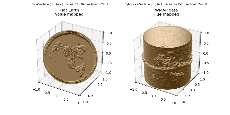
The image pixel data is used to map color values to geometry. For the left image, the value color component was used (the default component). For the right image, the hue color component was used by setting cref to ‘h’. Using the hzero parameter, the start value is blue (0.7) and increases in a negative direction going from blue to cyan, green, and finally red.

from matplotlib import pyplot as plt
import s3dlib.surface as s3d
import s3dlib.cmap_utilities as cmu

#.. Image Geometric Mapping

# 2. Setup and map surfaces .........................................
rez = 6
cmu.rgb_cmap_gradient( [0.25,0.15,0], [1,.9,.75], 'cardboard' )

earthElev = s3d.PolarSurface(rez)
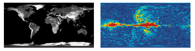
earthElev.map_geom_from_image('data/elevation.png', 0.075)
earthElev.transform(scale=1.2, rotate=s3d.eulerRot(45,45,180))
earthElev.map_cmap_from_normals(cmap='cardboard',direction=[-1,1,1])

WMAPelev = s3d.CylindricalSurface(rez)
WMAPelev.map_geom_from_image('data/wmap_2.png', 0.15, cref='h', hzero=-0.7)
WMAPelev.transform(rotate=s3d.eulerRot(135,0))
WMAPelev.map_cmap_from_normals(cmap='cardboard',direction=[-1,1,1])

# 3. Construct figures, add surfaces, and plot .....................

fig = plt.figure(figsize=plt.figaspect(0.5))
fig.text(0.47,0.975,str(earthElev), ha='right', va='top', fontsize='smaller')
fig.text(0.9,0.975,str(WMAPelev), ha='right', va='top', fontsize='smaller', multialignment='right')

ax1 = fig.add_subplot(121, projection='3d')
ax2 = fig.add_subplot(122, projection='3d')
minmax = (-1,1)
ax1.set(xlim=minmax, ylim=minmax, zlim=minmax, aspect='equal')
ax2.set(xlim=minmax, ylim=minmax, zlim=minmax, aspect='equal')
ticks=[-1,-.5,0,.5,1]
ax1.set_xticks(ticks)
ax1.set_yticks(ticks)
ax1.set_zticks(ticks)
ax2.set_xticks(ticks)
ax2.set_yticks(ticks)
ax2.set_zticks(ticks)
ax1.set_title('Flat Earth\nValue mapped')
ax2.set_title('WMAP data\nHue mapped')

ax1.add_collection3d(earthElev)
ax2.add_collection3d(WMAPelev)

plt.show()