Transparent Cloud Sections

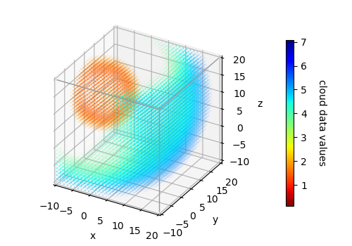
To emphasize values within a point cloud, a colormap is constructed starting with a list to set the alpha values of a colormap. The list is then used to define a linear segmented function, op_List, using the function linsegfunc. Finally, this function is applied to construct the following colormap using the colormap routine op_alpha_cmap.

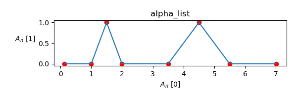
where the distribution of alpha values is shown below.

Since the Matplotlib colorbars cannot directly show transparencies, the opaque colormap is used, as shown in the highlighted lines below.

import numpy as np
import matplotlib.pyplot as plt
import s3dlib.surface as s3d
import s3dlib.cmap_utilities as cmu
import matplotlib.cm as cm
import matplotlib.colors as mcolors

# 1. Generate a spherical cloud distribution to examine ............
N,rng = 30, 3   # cloud divisions & the spherical function domain.
x,y,z = np.mgrid[ -rng:rng:N*1j,-rng:rng:N*1j,-rng:rng:N*1j ]
x,z = x+2, z-1   # offset spherical distribution
cloud = np.sqrt(x**2 + y**2 + z**2)

domain,cmap = [-10,20], 'jet_r'   # xyz domain to interpret the cloud

alpha_list = [ [0.13,0.0],[1.0,0.0],[1.5,1.0],[2.0,0.0], 
               [3.5,0.0], [4.5,1.0], [5.5,0.0], [7.01,0.0] ]
op_list = lambda t : cmu.linsegfunc(t, alpha_list)
cmu.op_alpha_cmap(cmap,op_list, name='mapL')

# 2. Setup data ....................................................
xyz, colors, _ = s3d.get_points_from_cloud(cloud,domain,'mapL')
norm = mcolors.Normalize(np.min(cloud),np.max(cloud) )
scmp = cm.ScalarMappable(norm=norm,cmap=cmap)

# 3. Construct figures, add points, and plot .......................
fig = plt.figure(figsize=(5,3.5))
mnx = domain
ax = fig.add_subplot(111, projection='3d', aspect='equal',proj_type='ortho')
ax.set(xlim=mnx,ylim=mnx,zlim=mnx,xlabel='x',ylabel='y',zlabel='z')

ax.scatter(*xyz, c=colors, marker='.', s=2)
cbar = plt.colorbar(scmp, ax=ax,  shrink=0.8, pad=.15 )
cbar.set_label('cloud data values', rotation=270, labelpad = 20)

vE,iE = [ [-10,-10,20], [20,-10,20], [20,20,20], [20,-10,-10] ], [ [0,1,2],[1,3]]
ax.add_collection3d( s3d.ColorLine3DCollection(vE,iE,color='0.6',lw=1) )

fig.tight_layout(pad=2)
plt.show()