Lab Colormaps

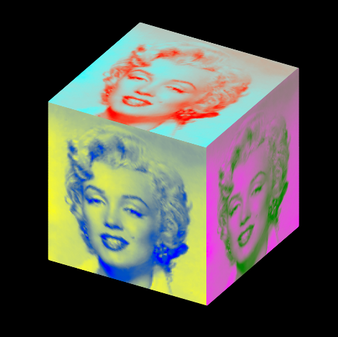
A grey scale image was colored using a Lab gradient colormap to preserve the visual contrast in the Monroe photo . The image contrast was first used to vary the vertical coordinates of the planar surface. This was then colorized by applying the colormap to surface geometry in the vertical direction. Finally the surface was flattened and rotated into position.

import copy
import numpy as np
import matplotlib as mpl
import matplotlib.pyplot as plt
import s3dlib.surface as s3d
import s3dlib.cmap_xtra as cmx

# Lab colormaps

# 2. Setup and map surface .........................................
rez = 6

cmx.Lab_cmap_gradient('blue', 'yellow', name='Lab_by')
cmx.Lab_cmap_gradient('red',  'cyan',   name='Lab_rc')
cmx.Lab_cmap_gradient('green','magenta',name='Lab_gm')
cmaps = [ 'Lab_by', 'Lab_rc', 'Lab_gm' ]     # <-- Linear in L*
#cmaps = [ 'viridis', 'plasma', 'inferno' ]  # <-- Perceptually Uniform Sequential

rot_by = lambda c: [c[0], -np.ones(len(c[0])), c[1]]
rot_rc = lambda c: [c[0], c[1],                np.ones(len(c[0])) ]
rot_gm = lambda c: [np.ones(len(c[0])), c[0],  c[1] ]
rotop = [  rot_by ,  rot_rc,   rot_gm  ]

photo = s3d.PlanarSurface(rez, basetype='oct1')
photo.map_geom_from_image('data/Monroe.png')

# 3. Construct figure, add surface plot ............................

minmax=(-1.07,1.07)
fig = plt.figure(figsize=plt.figaspect(1), facecolor='black')
ax = plt.axes(projection='3d', facecolor='black', aspect='equal')
ax.set(xlim=minmax, ylim=minmax, zlim=minmax)
ax.set_axis_off()
ax.set_proj_type('ortho')

for i in range(3) :
    surface = copy.copy(photo)
    surface.map_cmap_from_op( cmap=cmaps[i] )
    surface.map_geom_from_op( rotop[i] )
    ax.add_collection3d(surface)

fig.tight_layout(pad=0)
plt.show()

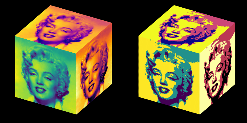
Posterization of the image is achieved by using a colormap of fewer colors as shown below:

using the following colormaps:

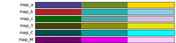
The colors for the cmapsABC colormaps were selected with increasing L* values (see the CSS colors table). The cmapsYCM colormaps are linear in L* with a constant Hue using the Hue_Lab_gradient function. The lightness for these colormaps is shown below:

import copy
import numpy as np
import matplotlib.pyplot as plt
import s3dlib.surface as s3d
import s3dlib.cmap_xtra as cmx
import s3dlib.cmap_utilities as cmu

# Warhol colormaps

# 2. Setup and map surface .........................................
rez = 6

cmu.stitch_color('darkslateblue','olivedrab',    'gold',    name="map_a")   # L*: 33,57,89
cmu.stitch_color('firebrick',    'lightseagreen','skyblue', name="map_b")   # L*: 44,67,81
cmu.stitch_color('darkgreen',    'cadetblue',    'thistle', name="map_c")   # L*: 37,63,83
cmapsABC = [ 'map_a', 'map_b', 'map_c' ]

N=3
cmu.stitch_color(*cmx.Hue_Lab_gradient('yellow' )(np.linspace(.3,.9,N)), name="map_Y")
cmu.stitch_color(*cmx.Hue_Lab_gradient('cyan'   )(np.linspace(.3,.9,N)), name="map_C")
cmu.stitch_color(*cmx.Hue_Lab_gradient('magenta')(np.linspace(.3,.9,N)), name="map_M")
cmapsYCM = [ 'map_Y', 'map_C', 'map_M' ]

rot_by = lambda c: [c[0], -np.ones(len(c[0])), c[1]]
rot_rc = lambda c: [c[0], c[1],                np.ones(len(c[0])) ]
rot_gm = lambda c: [np.ones(len(c[0])), c[0],  c[1] ]
rotop = [  rot_by ,  rot_rc,   rot_gm  ]

photo = s3d.PlanarSurface(rez, basetype='oct1')
photo.map_geom_from_image('data/Monroe.png')

# 3. Construct figure, add surface plot ............................

minmax=(-1,1)
fig = plt.figure(figsize=(8,4), facecolor='black')

cmapSet = [ cmapsABC,cmapsYCM]
for j,cmaps in enumerate(cmapSet) :
    ax = fig.add_subplot(121+j, projection='3d', aspect='equal')
    ax.set(xlim=minmax, ylim=minmax, zlim=minmax)
    ax.set_facecolor('black')
    ax.set_axis_off()
    ax.set_proj_type('ortho')

    for i in range(3) :
        surface = copy.copy(photo)
        surface.map_cmap_from_op( cmap=cmaps[i] )
        surface.map_geom_from_op( rotop[i] )
        ax.add_collection3d(surface)

fig.tight_layout(pad=0)
plt.show()

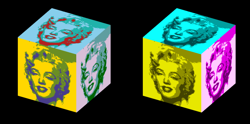
Similarly, the photo may be visualized using any linear L* colormap. Using the Matplotlib ‘Perceptually Uniform Sequential* colormaps, define the colormaps:

from matplotlib.colors import ListedColormap
from matplotlib import colormaps

viridis3 = ListedColormap(colormaps['viridis'](np.linspace(0, 1, 3)))
plasma3  = ListedColormap(colormaps['plasma'](np.linspace(0, 1, 3)))
inferno3 = ListedColormap(colormaps['inferno'](np.linspace(0, 1, 3)))
cmapsABC  = [ 'viridis', 'plasma', 'inferno' ]
cmapsYCM  = [ viridis3, plasma3, inferno3 ]

Then the previous code produces the following figure: