Unstructured Planar Dataset

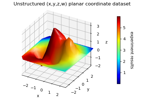
This example is similar to the Unstructured coordinates, Smoothed Surface example with the addition of scalar values assigned to each vertex. When creating the object, the vertex coordinate array may includes the vertex values. Without values, the array shape for N vertices is (N,3). When vertex values are included, the shape is (N,4). The functions used to describe the geometry are from the Matplotlib 2D examples Unstructured coordinates and Tricontour Smooth Delaunay .

Smoothed colormapping uses these vertex values following Surface Triangulation. The surface visualizations are enhanced with shading for the argument flat=False.

import numpy as np
import matplotlib.pyplot as plt
import s3dlib.surface as s3d

# 1. Create dataset to examine from matplotlib examples ..............

def experiment_res(x, y):
    """An analytic function representing experiment results."""
    x = 2 * x
    r1 = np.sqrt((0.5 - x)**2 + (0.5 - y)**2)
    theta1 = np.arctan2(0.5 - x, 0.5 - y)
    r2 = np.sqrt((-x - 0.2)**2 + (-y - 0.2)**2)
    theta2 = np.arctan2(-x - 0.2, -y - 0.2)
    z = (4 * (np.exp((r1/10)**2) - 1) * 30 * np.cos(3 * theta1) +
         (np.exp((r2/10)**2) - 1) * 30 * np.cos(5 * theta2) +
         2 * (x**2 + y**2))
    return (np.max(z) - z) / (np.max(z) - np.min(z))

np.random.seed(3)
x = np.random.uniform(-3, 3, 256)
y = np.random.uniform(-3, 3, 256)
z = (1 - x/2 + x**5 + y**3) * np.exp(-x**2 - y**2)
z=3*z
w = 6*experiment_res(x/3,y/3)  # <-- include vertex values

# z,w = w,z  <-- uncomment to switch z,w alternative surface views
xyzw = np.array([x,y,z,w])
xyz = np.array([x,y,z])  # <-- for scatter plot

# 2. Setup and map surfaces .........................................
surface = s3d.PlanarSurface.pntsurf(xyzw.T)
surface.triangulate(4)
surface.map_cmap_from_vertvals('jet')

# 3. Construct figure, add surface, plot ............................
fig = plt.figure(figsize=(5,3.5))
figTitle = 'Unstructured (x,y,z,w) planar coordinate dataset'
fig.text(0.5,0.98,figTitle, ha='center', va='top', fontsize='large')
ax = plt.axes(projection='3d', aspect='equal',proj_type='ortho')
ax.set(xlabel='x',ylabel='y',zlabel='z')

s3d.auto_scale(ax,surface,uscale=0.8)
ax.add_collection3d(surface.shade( flat=False).hilite(.6,flat=False, focus=2) )

cbar = plt.colorbar(surface.cBar_ScalarMappable,ax=ax,shrink=0.8, pad=.15 )
cbar.set_label('experiment results', rotation=270, labelpad=20)

fig.tight_layout(pad=2)
plt.show()

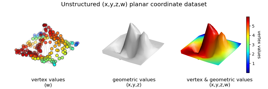
The separate structure of the above plot can be illustrated as shown below:

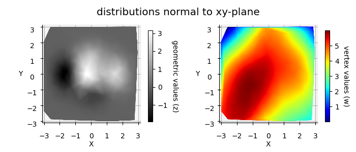
The 2D plot can be visualized by rotating the plot using ax.view_init(90,-90) and omitting any surface shading.

The colormapping for the above left and right plots was for the vertical position and vertex values, respectively, as given by:

surface_Z.map_cmap_from_op(cmap='binary_r')
surface_W.map_cmap_from_vertvals('jet')

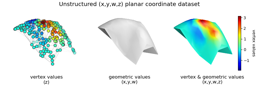
For a planar xy-dataset, z and w are the dependent values. Thus, either z or w can represent the vertical direction or vertex value. By simply inserting the line:

z,w = w,z

the previous representation is reversed, producing: