Jacksboro Fault

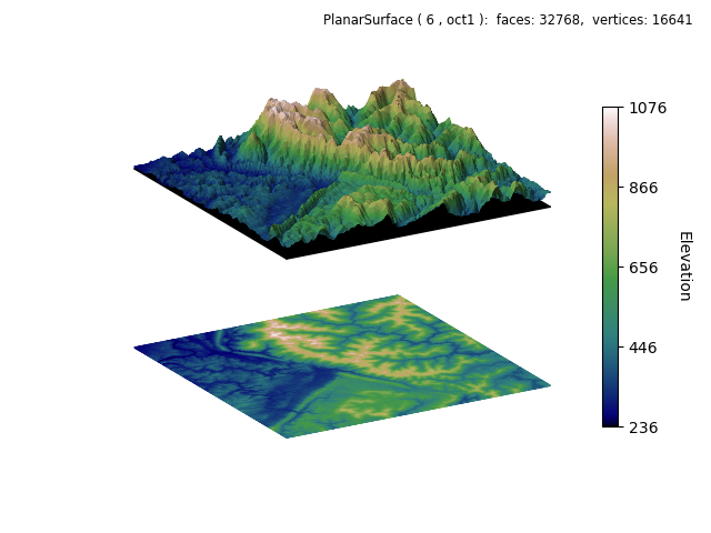
This figure is an 3D representation for Topographic_hillshading AMatplotlib example. When projected normal to the x-y plane, it is similar to the Matplotlib example.

The Matplotlib example demonstrates various hillshading controls. In this example, 3D effects are controlled by the surface method arguments:

• the scale argument of the map_geom_from_datagrid method. This is analogous to the Matplotlib vertical exaggeration.
• the shade method arguments, as described in the Shading, Highlighting and Color Mapped Normals guides.
  • the depth argument, which controls the maximum ‘darkness’ of the shading.
  • the direction argument, which controls the ‘sun’ Matplotlib location.
  • the contrast argument, which controls the relative contrast of shading.

For this example case, the argument values were selected based on the 3D representation, not the 2D view.

import copy
import numpy as np
import matplotlib.pyplot as plt
import s3dlib.surface as s3d

#.. Geometric and Color Datagrid Mapping, 2

# 1. Define function to examine .....................................

Z=np.load('data/jacksboro_fault_dem.npz')['elevation']
datagrid = np.flip(Z,0)

# 2. Setup and map surfaces .........................................
rez=6

surface = s3d.PlanarSurface(rez, basetype='oct1', cmap='gist_earth')
surface.map_cmap_from_datagrid( datagrid )
surface.map_geom_from_datagrid( datagrid, scale=0.35 )

surface.transform(translate=[0,0,0.5])  # move up to 0.5
flat_surf = copy.copy(surface)
# flatten and move down to -0.75
flat_surf.map_geom_from_op(lambda c: [c[0],c[1],-0.75*np.ones_like(c[0])] )

# 3. Construct figure, add surface, plot ............................

fig = plt.figure()
fig.text(0.975,0.975,str(surface), ha='right', va='top',
        fontsize='smaller', multialignment='right')
ax = plt.axes(projection='3d', aspect='equal')
ax.set(xlim=(-1,1), ylim=(-1,1), zlim=(-1,1) )
minc, maxc = surface.bounds['vlim']
cbar=plt.colorbar(surface.cBar_ScalarMappable, ax=ax,
        ticks=np.linspace(minc,maxc,5), shrink=0.6, pad=0  )
cbar.set_label('Elevation', rotation=270, labelpad = 15)
ax.set_axis_off()
ax.set_proj_type('ortho')
ax.view_init(elev=20, azim=60)

surface.shade(depth=0,direction=(1,0,1),contrast=1.3)
ax.add_collection3d(surface)
ax.add_collection3d(s3d.PlanarSurface(color='k').domain(zcoor=0.5))
ax.add_collection3d(flat_surf)

fig.tight_layout(pad=0)
plt.show()

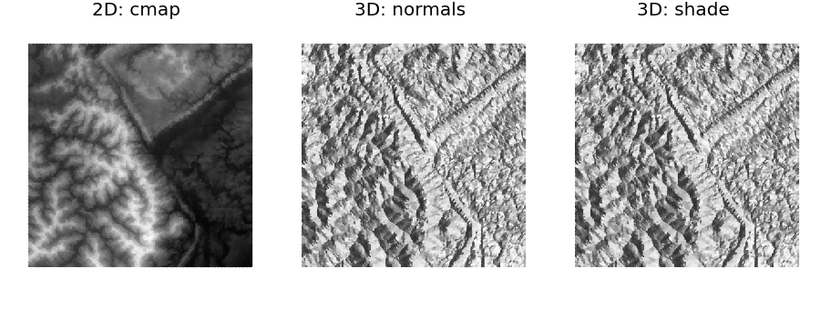
Alternatively, the 3D effect on the 2D view can be created from the surface map_cmap_from_normals method. This is demonstrated below using a grey scale.

import numpy as np
import matplotlib.pyplot as plt
import s3dlib.surface as s3d
import copy
#.. Geometric and Color Datagrid Mapping, 3

# 1. Define function to examine .....................................

Z=np.load('data/jacksboro_fault_dem.npz')['elevation']
datagrid = np.flip(Z,0)

# 2. Setup and map surfaces .........................................
rez=6

flatsurface = s3d.PlanarSurface(rez, basetype='oct1')
flatsurface.map_cmap_from_datagrid( datagrid, cmap='binary_r' )

surface3D = s3d.PlanarSurface(rez, basetype='oct1', color='w')
surface3D.map_geom_from_datagrid( datagrid )

surfaces = [ flatsurface, surface3D, copy.copy(surface3D) ]
title = [ '2D: cmap', '3D: normals', '3D: shade' ]
# 3. Construct figure, add surface, plot ............................

fig = plt.figure(figsize=(9,3.5))
minmax=(-.7,.7)
for i,surface in enumerate(surfaces) :
    ax = fig.add_subplot(131+i, projection='3d', aspect='equal')
    ax.set(xlim=minmax, ylim=minmax, zlim=minmax )
    ax.set_axis_off()
    ax.set_proj_type('ortho')
    ax.view_init(90,-90)
    ax.set_title(title[i], fontsize='x-large')

    if   i==0  : pass
    elif i==1  : surface.map_cmap_from_normals(cmap='binary_r')
    else :       surface.shade()
    ax.add_collection3d(surface)

fig.tight_layout(pad=0)
plt.show()