Color Space

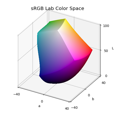
For the Lab surface, the RGB cube is directly defined in xyz space. Then, the coordinates are directly converted to Lab space using the colorspacious package.

from matplotlib import pyplot as plt
import s3dlib.surface as s3d
from colorspacious import cspace_converter

#.. Lab Color Space

# 1. Define function to examine ....................................

def rgb_to_labCoor(rgb):
    L,a,b = cspace_converter("sRGB1", "CAM02-UCS"  )(rgb.T).T
    return a,b,L

# 2. Setup and map surface .........................................

surface = s3d.CubicSurface().domain([0,1],[0,1],[0,1]).triangulate(6)
surface.map_color_from_op(lambda xyz : xyz)
surface.map_geom_from_op(rgb_to_labCoor)

# 3. Construct figure, add surface plot ............................

fig = plt.figure(figsize=plt.figaspect(1))
ax = plt.axes(projection='3d', aspect='equal')
ax.set( xlim=(-40,40),     ylim=(-40,40),     zlim=(0,100),
        xlabel='a',        ylabel='b',        zlabel='L', 
        xticks=[-40,0,40], yticks=[-40,0,40], zticks=[0,50,100])
ax.set_title( 'sRGB Lab Color Space', fontsize='x-large' )
ax.set_proj_type('ortho')

ax.add_collection3d(surface.shade())

fig.tight_layout()
plt.show()

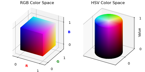
For the RGB and HSV surfaces, a unit surface is set in the native color space coordinate system and color mapped directly.

import numpy as np
import matplotlib.pyplot as plt
import s3dlib.surface as s3d

#.. RGB and HSV Color Spaces

# 1. Define functions to examine ....................................

def hsvColor(rtz) :
    r,t,z = rtz
    return t/(2*np.pi), r, z  # all values are in [0,1]

# 2. Setup and map surfaces .........................................
rez = 5

rgb_cube = s3d.CubicSurface(rez).domain([0,1],[0,1],[0,1])
rgb_cube.map_color_from_op(lambda xyz : xyz)

hsv_cyl = s3d.CylindricalSurface(rez,'squ_v').domain(1,[0,1])
hsv_cyl.map_color_from_op(hsvColor,rgb=False)

# 3. Construct figure, add surfaces, and plot .....................

hsv_minmax = (-1.3,1.3)
rgb_minmax, rgb_ticks = (-0.2,1.2) , [0,1]
fig = plt.figure(figsize=(6,3))

ax1 = fig.add_subplot(121, projection='3d', aspect='equal')
ax1.set(xlim=rgb_minmax,  ylim=rgb_minmax,  zlim=rgb_minmax,
        xticks=rgb_ticks, yticks=rgb_ticks, zticks=rgb_ticks)
ax1.set_xlabel('R', labelpad=-10, color='r', fontweight='bold')
ax1.set_ylabel('G', labelpad=-10, color='g', fontweight='bold')
ax1.set_zlabel('B', labelpad=-10, color='b', fontweight='bold')
ax1.set_title( 'RGB Color Space' )
ax1.set_proj_type('ortho')

ax2 = fig.add_subplot(122, projection='3d', aspect='equal')
ax2.set(xlim=hsv_minmax, ylim=hsv_minmax, zlim=(0,1),
        xticks=[],       yticks=[0],      zticks=[0,1])
ax2.set_zlabel('Value', labelpad=-10)
ax2.set_title( 'HSV Color Space' )
ax2.set_proj_type('ortho')

ax1.add_collection3d(rgb_cube.shade(.5))
ax2.add_collection3d(hsv_cyl.shade(.5))

fig.tight_layout()
plt.show()

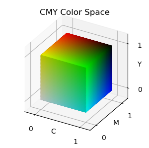
By simply changing the above highlighted line for the cube object as:

rgb_cube.map_color_from_op(lambda xyz : 1-xyz)

the CMY color space is created, as shown below