Wireframe Plots

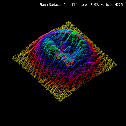
Mapping function are similarly defined as in the Geeks3D examples. Here, the only difference is the use of Numpy arrays. The following custom color map was used for the visualization.

A triangular face surface object, PlanarSurface with a basetype ‘oct1’ was used for the above plot.

For displaying a rectangular grid, use the following instead:

surface = s3d.PlanarSurface(rez,basetype='squ',linewidth=.3)

For both cases, edge colors are derived from the surface colors which have transparent facecolor. Using this approach, shading and highlighting are included in the edge color visualization.

Alternatively, using the surface.edge line object would require color mapping of the line. However, shading and highlighting would not be available for the edge line object.

import numpy as np
import matplotlib.pyplot as plt
import s3dlib.surface as s3d
import s3dlib.cmap_utilities as cmu  

#.. Surface Wireframe plot 

# 1. Define function to examine .....................................

def fun011(xyz) :
    x,y,z = xyz
    X2, Y2 = x**2, y**2
    a,b = 0.04, 0.06
    R2 = a*X2 + b*Y2
    one = np.ones(len(x))
    f = np.sin( X2 + 0.1*Y2)/( 0.1*one + R2 )
    g = ( X2 + 1.9*Y2) * np.exp( one - R2)/4
    Z = f + g
    return x,y,Z

# 2. Setup and map surfaces .........................................
rez=5
cmap = cmu.hsv_cmap_gradient([1.166,1,1],[0.333,1,1],name='yel_grn')

surface = s3d.PlanarSurface(rez,basetype='oct1',linewidth=.2).domain(10,10)
surface.map_geom_from_op(fun011)
surface.map_cmap_from_op(lambda xyz : np.abs(fun011(xyz)[2]), cmap )
#surface.map_cmap_from_op(cmap=cmap)  # alternative, using the geometry (planar default)
surface.shade(.5).hilite(.3)
surface.set_facecolor([0,0,0,0])

# 3. Construct figures, add surface, plot ...........................

fig = plt.figure(figsize=plt.figaspect(1), facecolor='black')
fig.text(0.975,0.975,str(surface), ha='right', va='top',
        fontsize='smaller', multialignment='right', color='white')
ax = plt.axes(projection='3d', aspect='equal')
minmax = (-9,9)
ax.set(xlim=minmax, ylim=minmax, zlim=minmax)
ax.set_axis_off()
ax.set_facecolor('black')
ax.set_proj_type('ortho')
ax.view_init(50,140)

ax.add_collection3d(surface)

fig.tight_layout()
plt.show()

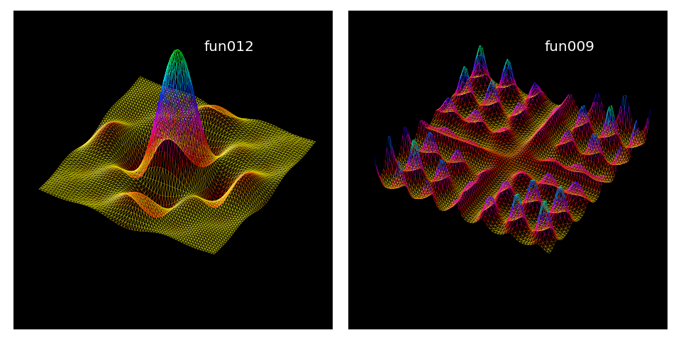
Further examples of viewing only edges are shown below. Surface objects were identically constructed as in the previous script with only changes made to the function references.

# 1. Define function to examine .....................................

def fun009(xyz) :
    x,y,z = xyz
    a,b,c = 1,1,15
    lim = 0.001  # use L'Hopital's rule as x -> 0
    A = np.where(np.abs(x)<lim, np.ones(len(x)), np.divide( np.sin(a*x), a*x ) )
    B = np.where(np.abs(y)<lim, np.ones(len(y)), np.divide( np.sin(b*y), b*y ) )
    Z  = c*A*B
    return x,y,Z

def fun012(xyz) :
    x,y,z = xyz
    A = 0.9*np.exp( np.sin(2*x)*np.sin(0.2*y))
    B = 0.9*np.exp( np.sin(2*y)*np.sin(0.2*x))
    Z  = A*B
    return x,y,Z