
3D Demo
Mapping function definition was taken from the Mayavi demo example.
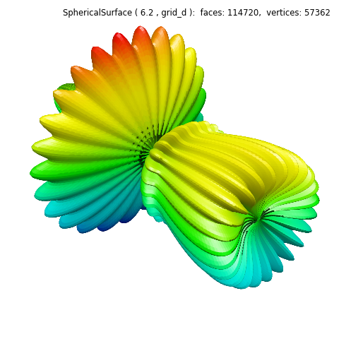
The functional definition given in the Mayavi reference, combined with the base surface face ‘right-hand rule’ definition, produces faces having normals which point inward. Using this definition, the produced figure would appear as follows.
To produce a surface ‘in-side out’, the evert method was used to reverse the normals, as shown in the highlighted line in the following script. Also, custom color map was used to create a similar visualization

This S3Dlib example demonstrates the limitations of using the predefined surface grids. Here, the visualization anomalies are along surface faces near the axis of symmetry. These anomalies could be minimized by increasing the number of faces in the constructor. (This demo uses 240 angular increments, the same as the Mayavi demo) The tradeoff is increasing rendering time.
import numpy as np
import matplotlib.pyplot as plt
import s3dlib.surface as s3d
import s3dlib.cmap_utilities as cmu

#.. 3D Surface Plot

# 1. Define function to examine .....................................

def mayDemo(rtp) :
    r,theta,phi = rtp
    m0 = 4; m1 = 3; m2 = 2; m3 = 3; m4 = 6; m5 = 2; m6 = 6; m7 = 4;
    R = np.sin(m0*phi)**m1 + np.cos(m2*phi)**m3 + np.sin(m4*theta)**m5 + np.cos(m6*theta)**m7
    x = R*np.sin(phi)*np.cos(theta)
    y = R*np.cos(phi)
    z = R*np.sin(phi)*np.sin(theta)
    return [x,y,z]

def zAxisDir(rtp) : return s3d.SphericalSurface.coor_convert(rtp,True)[2]

# 2. Setup and map surfaces .........................................
cmap = cmu.hue_cmap('b','r',2.0,name='BlRd')
illum = s3d.rtv([1,0,0.75],35,48)

surface = s3d.SphericalSurface.grid(10*24,10*24)
surface.map_geom_from_op(mayDemo,True).evert()
surface.map_cmap_from_op(zAxisDir,cmap)

# 3. Construct figures, add surface, plot ...........................

fig = plt.figure(figsize=plt.figaspect(1))
fig.text(0.975,0.975,str(surface), ha='right', va='top',
        fontsize='smaller', multialignment='right')
ax = plt.axes(projection='3d', aspect='equal')
ax.set(xlim=(-1.2,1.2), ylim=(-0.8,1.6), zlim=(-1.2,1.2))
ax.view_init(35,48)
ax.set_axis_off()

ax.add_collection3d(surface.shade(0.1,illum).hilite(.7,illum,focus=2))

fig.tight_layout()
plt.show()