Complex Number Representation, Radius and Angle

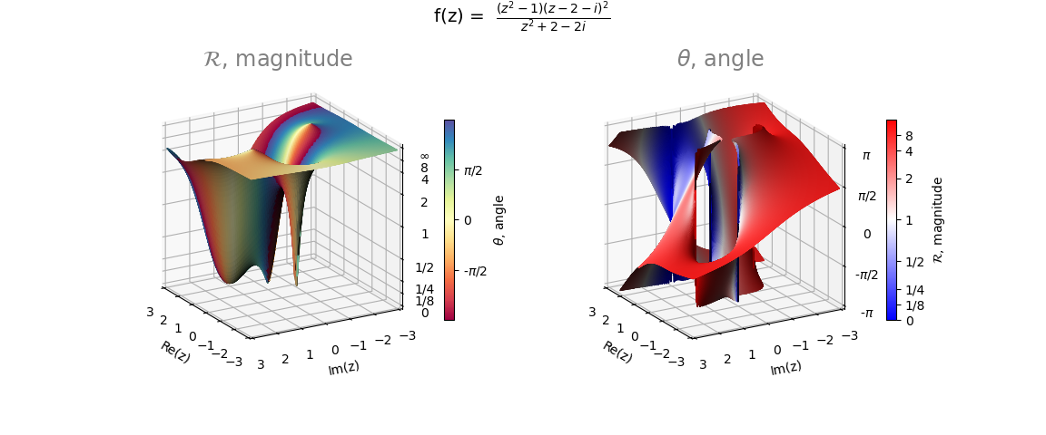
For this case, the Euler representation of a complex number:

re^iθ = r(cosθ + isinθ) ,

was used to visualize a complex function for r and θ surfaces (instead of real and imaginary, as was in the Functions having a Singularity example ).

The function require several specific algorithmic constructions to create the surface 3D visualizations within the domain of interest:

1. Several singularities exist for the radial magnitude. The following was used to provide a range between zero and one.
   ℛ(r) = 2arctan(r)/π
   This is shown in the highlighted code.
2. Several discontinuities are present in the angle surface. Surface faces in the region of the discontinuities have normals ‘approximately’ in the horizontal plane. These faces were ‘clipped’ out of the surface, indicated in the highlighted code.

import numpy as np
from matplotlib import pyplot as plt
import s3dlib.surface as s3d

#.. Radial/Angular Complex Function Visualization

# 1. Define function to examine .....................................
def complexFunc(z):
    # https://en.wikipedia.org/wiki/Domain_coloring
    i = 1j
    num = (z**2 - 1)*(z - 2 -i)**2
    dem = z**2 + 2 + 2*i
    return num/dem

def funcRT(xyz) :
    x,y,z = xyz
    c = np.array(x,dtype=complex)
    c.imag = np.array(y)
    f = complexFunc(c)
    r = np.abs(f)
    Z = 2*np.arctan(r)/np.pi           #.. [0,1]
    theta = (1 + np.angle(f)/np.pi)/2  #.. [0,1]
    return Z,theta 

coor_radius  = lambda c: [c[0],c[1],funcRT(c)[0]]
coor_theta   = lambda c: [c[0],c[1],funcRT(c)[1]]
isContinuous = lambda c,N: np.abs(N.T[2]) > 0.02

# 2. Setup and map surfaces .........................................
rez = 6

surfaces = [None]*2
surface = s3d.PlanarSurface(rez,cmap='Spectral').domain([-3,3],[-3,3])
surface.map_cmap_from_op( lambda c: funcRT(c)[1] )
surface.map_geom_from_op( coor_radius )
surfaces[0]=surface

# note: higher rez due to surface discontinuity.
surface = s3d.PlanarSurface(rez+2,cmap='bwr').domain([-3,3],[-3,3])
surface.map_cmap_from_op( lambda c: funcRT(c)[0] )
surface.map_geom_from_op( coor_theta )
normals = surface.facenormals(v3d=False)
surface.clip(lambda c : isContinuous(c,normals)) # remove discontinuous faces
surfaces[1]=surface

# 3. Construct figure, add surface, plot ............................
elev,azim = 20,150

r_labels = [ '0','1/8','1/4','1/2','1','2','4','8',r'$\infty$']
r_axvals = [0] + [ 2*np.arctan(2**i)/np.pi for i in range(-3,4)] + [1]
t_labels = [r'-$\pi$',r'-$\pi$/2','0',r'$\pi$/2',r'$\pi$']
t_axvals = [ v/4 for v in range(0,5)]
z_ticks = [r_axvals,t_axvals]
z_axlab = [r_labels,t_labels]
title = [ r'$\mathcal{R}$, magnitude', r'$\theta$, angle']

fig = plt.figure(figsize=plt.figaspect(0.5/1.2))
info = r" f(z) =  $\frac{(z^{2}-1)(z-2-i)^{2}}{z^{2}+2-2i}$  "
fig.text(0.5,1,info, ha='center', va='top', fontsize='x-large')
for i,surface in enumerate(surfaces) :
    ax = fig.add_subplot(121+i, projection='3d',aspect='equal')
    ax.view_init(elev,azim)
    ax.set_proj_type('ortho')
    ax.set_title('\n'+title[i],color='grey', fontsize='xx-large', pad=-1)
    ax.set(xlim=( -3,3 ), ylim=( -3,3 ), zlim=( 0,1), zticks=z_ticks[i],
                xlabel='Re(z)', ylabel='Im(z)' )
    ax.set_zticklabels(z_axlab[i])
    cbar = plt.colorbar(surface.cBar_ScalarMappable, ax=ax, ticks=z_ticks[1-i], shrink=0.6 )
    cbar.ax.set_yticklabels(z_axlab[1-i])
    cbar.set_label(title[1-i], rotation=90)
    
    surface.shade(0.0,ax=ax,direction=[0.5,1,1])
    if i==1 : surface.hilite(.8,direction=[0,1,1],focus=1)
    ax.add_collection3d(surface)

plt.show()