Functions having a Singularity

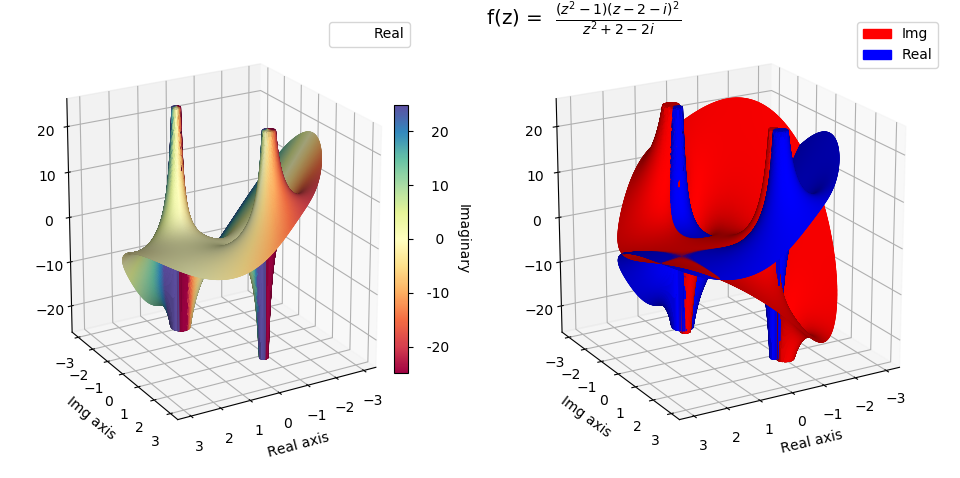
In this example, the function has several singularities within the domain. Plotting such functions may be accomplished using three different approaches:

1. the function may be defined with an upper limit to the evaluation. The result is a ‘flattened’ surface in the region of the singularity. This was the approach taken for this example and is indicated in the highlighted line in the following source code.
2. Once the surface is constructed, the surface may be ‘clipped’ using a bounding function. The resulting surface will have ‘holes’ in the region of the singularity.
3. The function evaluation may be further transformed to a limited range. This approach is exemplified in Complex Number Representation, Radius and Angle .

import numpy as np
import matplotlib.pyplot as plt
import matplotlib.patches as mpatches
import matplotlib.lines as mlines
from matplotlib.ticker import LinearLocator, FormatStrFormatter
import s3dlib.surface as s3d

#.. Real/Imag Complex Function Visualization

# 1. Define functions to examine ....................................
domainR,maxZ = 3,25

def complexFunc(z):
    # https://en.wikipedia.org/wiki/Domain_coloring
    i = 1j
    num = (z**2 - 1)*(z - 2 -i)**2
    dem = z**2 + 2 + 2*i
    return num/dem

def real_imagFunc(rtz,isReal):
    r,t,z = rtz
    x,y = r*np.cos(t), r*np.sin(t)
    c = np.array(x,dtype=complex)
    c.imag = np.array(y)
    f = complexFunc(c)
    Z = f.real if isReal else f.imag
    Z = np.where(np.abs(Z) > maxZ, maxZ*np.sign(Z), Z ) # flatten  
    return r,t,Z

real = True
imaginary =  not real

# 2. Setup and map surfaces .........................................
rez = 7

surfaces = [None]*2
surface = s3d.PolarSurface(rez, cmap='Spectral').domain(domainR)
surface.map_cmap_from_op( lambda rtz : real_imagFunc(rtz,imaginary)[2] )
surface.map_geom_from_op( lambda rtz : real_imagFunc(rtz,real) )
surfaces[0] = surface

surface_I = s3d.PolarSurface(rez, facecolor='red').domain(domainR)
surface_I.map_geom_from_op( lambda rtz : real_imagFunc(rtz,imaginary) )
surface_R = s3d.PolarSurface(rez, facecolor='blue').domain(domainR)
surface_R.map_geom_from_op( lambda rtz : real_imagFunc(rtz,real) )
surfaces[1] = surface_I + surface_R

# 3. Construct figure, add surfaces, and plot .....................

fig = plt.figure(figsize=plt.figaspect(0.6/1.2))
info = r" f(z) =  $\frac{(z^{2}-1)(z-2-i)^{2}}{z^{2}+2-2i}$  "
fig.text(0.5,1,info, ha='left', va='top', fontsize='x-large')
for i,surface in enumerate(surfaces) :
    ax = fig.add_subplot(121+i, projection='3d', aspect='equal')
    ax.view_init(20,60)
    ax.set_xlabel('Real axis')
    ax.set_ylabel('Img axis')
    if i==0 :
        cbar = plt.colorbar(surface.cBar_ScalarMappable, ax=ax,  shrink=0.6, pad=-.05 )
        cbar.set_label('Imaginary', rotation=270, labelpad = 15)
        cbar.ax.yaxis.set_major_formatter(FormatStrFormatter('%5.0f'))
        real_handle = mlines.Line2D([], [], color='grey', linestyle='None', label='Real')
        ax.legend(handles=[real_handle])
    else :
        red_patch = mpatches.Patch(color='red', label='Img')
        blue_patch = mpatches.Patch(color='blue', label='Real')
        ax.legend(handles=[red_patch,blue_patch])
    s3d.auto_scale(ax,surface)

    surface.shade(ax=ax,direction=[1,3,1])
    ax.add_collection3d(surface)

fig.tight_layout(pad=2)
plt.show()