Function Plots, z = f(x,y)

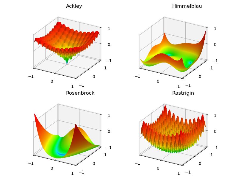
These examples show basic function plotting using:

one code statement to create a surface object, one code statement to create the surface geometry and one code statement to color the surface. Finally, one code statement to add that object to a Matplotlib 3D axis.

Also, several functions were used to demonstrate:

a functional relationship should look like a function

The functions are given on the Wikipedia page Test functions for optimization.

The following custom colormap was used for these visualizations.

import numpy as np
import matplotlib.pyplot as plt
import s3dlib.surface as s3d
import s3dlib.cmap_utilities as cmu  

#.. Function plots, z = f(x,y) 

# 1. Define functions to examine ....................................
# all functions normalized into the domain [-1.1]

def Ackley(xyz) :
    x,y,z = xyz
    X,Y = 5*x, 5*y
    st1 = -0.2*np.sqrt( 0.5*( X*X + Y*Y) )
    Z1 = -20.0*np.exp(st1)
    st2 = 0.5*( np.cos(2*np.pi*X) +  np.cos(2*np.pi*Y) )
    Z2 = -np.exp(st2) + np.e + 20
    Z = Z1 + Z2
    return x,y, Z/8 - 1

def Himmelblau(xyz) :
    x,y,z = xyz
    X,Y = 5*x, 5*y
    Z1 = np.square( X*X + Y - 11 )
    Z2 = np.square( Y*Y + X - 7  ) 
    Z = Z1 + Z2
    return x,y, Z/500 - 1

def Rosenbrock(xyz) :
    x,y,z = xyz
    X,Y = 2*x, 2*y+1
    Z1 = np.square( 1 - X )
    Z2 = 100*np.square( Y - X*X  ) 
    Z = Z1 + Z2
    return x,y, Z/1000 - 1

def Rastrigin(xyz) :
    x,y,z = xyz
    X,Y = 5*x, 5*y
    Z = 20 + X*X + Y*Y - 10*np.cos(2*np.pi*X) - 10*np.cos(2*np.pi*Y)
    return x,y, Z/40 - 1

# ..........................
def nonlinear_cmap(n) :
    # assume -1 < n < 1, nove to domain of [0,1]
    N = (n+1)/2
    return np.power( N, 0.1 )

# 2 & 3. Setup surfaces and plot ....................................
rez=6
cmap = cmu.hsv_cmap_gradient( 'b' , 'r' , smooth=0.8)
funcList = [ Ackley, Himmelblau, Rosenbrock, Rastrigin ]

minmax, ticks = (-1,1), (-1,0,1)
fig = plt.figure(figsize=(8,6))
for i in range(4) :
    # setup surfaces ....... 
    surface = s3d.PlanarSurface(rez,basetype='oct1')
    surface.map_geom_from_op(funcList[i])
    surface.map_cmap_from_op(lambda xyz :  nonlinear_cmap(xyz[2]), cmap )
    # ...................... 
    ax = fig.add_subplot(2,2,1+i, projection='3d')
    ax.set(xlim=minmax, ylim=minmax, zlim=minmax )
    ax.set_title(surface.name, fontsize='large', horizontalalignment='left')
    ax.set_xticks(ticks)
    ax.set_yticks(ticks)
    ax.set_zticks(ticks)
    ax.set_proj_type('ortho')
    ax.view_init(25)

    ax.add_collection3d(surface.shade(.5))

fig.tight_layout(pad=1)
plt.show()