Earth Elevation Projected Contours

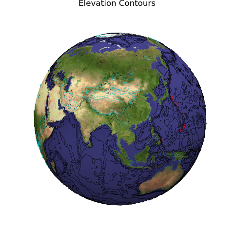
Similar to the Earth Elevation Contours example, contours are created from mapping the spherical geometry from an image, less the color mapping. In addition, the contours are projected back onto a sphere. The contours are clipped behind the viewing plane so as not to interfer with the underlying colored global sphere.

Since the view orientation is changed from the default elevation and azimuth, the direction of shading the globe is computed using the ‘relative to view’ method, rtv. The clipping plane direction is computed for the viewing elevation and azimuth using the elev_azim_2vector method.

Colormap for the contours:

from matplotlib import pyplot as plt
import s3dlib.surface as s3d
import s3dlib.cmap_utilities as cmu

#.. Earth Elevation Projected Contours

# 2. Setup and map surfaces .........................................
rez = 6
elev,azim = 25,-80
emap = cmu.stitch_color('r','k','c',bndry=[0.14,0.76],name='rkc')

globe = s3d.SphericalSurface(rez)
rtv = s3d.rtv([1,0,1], elev,azim)
globe.map_color_from_image('data/earth.png').shade(0.25,rtv)

earth = s3d.SphericalSurface(rez, cmap=emap)
earth.map_geom_from_image('data/earth_dry_elevation.png',0.3)
earth.map_cmap_from_op( )

earth_elev = earth.contourLineSet(8)  # default: spherical contours
earth_elev.map_to_plane(1.01,coor='s')
viewDir = -1*s3d.elev_azim_2vector(elev,azim)
earth_elev.clip_plane( 0, direction=viewDir )
earth_elev.set_linewidth(0.4)

# 3. Construct figure, add surfaces, and plot ......................

fig = plt.figure(figsize=plt.figaspect(1) )
ax = plt.axes(projection='3d', aspect='equal')
ax.set_title('Elevation Contours')
minmax = (-0.75,0.75)
ax.set(xlim=minmax, ylim=minmax, zlim=minmax)
ax.set_axis_off()
ax.view_init(elev,azim)

ax.add_collection3d(globe)
ax.add_collection3d(earth_elev)

fig.tight_layout(pad=0)
plt.show()