Line Slice Wireframe Plots

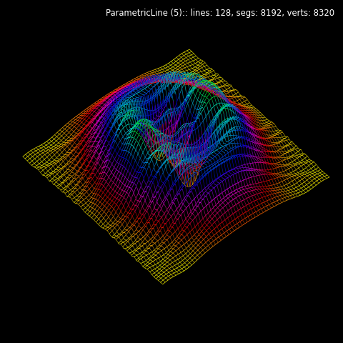
This example is similar to Wireframe Plots example, differing in construction methods and with minor image changes.

The functions used for the geometric mapping have a domain [-10,10]. As a result, the surface wireframe is constructed using edges from an initially colored surface which is scaled prior to geometric mapping. Since ParametricLine slices use a default domain for x and y as [-1,1], a xlim and ylim are used to set the domain for the slices. Then the lines are colormapped.

Visually, the surface wireframe shows the three edges of the triangular faces. Line slice plots will only show two ‘quadrilateral edges’. In addition, shading is more effective in surface wireframes with are based on the surface normals ( ParametricLines have no equivalent ‘normals’ property.)

Alternatively, a planar surface of a ‘grid’ base type could produce a similar result. The advantage of using slices is that number of ‘lines’ is set by xset and yset, not the rez of the planar surface. Also for the surface edges, the line segment would be straight. This is in contrast to line slices in which the resolution is set by the Parametric line rez.

import numpy as np
import matplotlib.pyplot as plt
import s3dlib.surface as s3d
import s3dlib.cmap_utilities as cmu  

#.. ParametricLine Wireframe plot 

# 1. Define function to examine .....................................

def fun011(xyz) :
    x,y,z = xyz
    X2, Y2 = x**2, y**2
    a,b = 0.04, 0.06
    R2 = a*X2 + b*Y2
    one = np.ones(len(x))
    f = np.sin( X2 + 0.1*Y2)/( 0.1*one + R2 )
    g = ( X2 + 1.9*Y2) * np.exp( one - R2)/4
    Z = f + g
    return x,y,Z

# 2. Setup and map surfaces .........................................
rez=5
cmap = cmu.hsv_cmap_gradient([1.166,1,1],[0.333,1,1])

line = s3d.ParametricLine(rez,lw=0.5)
line.map_xySlice_from_op( fun011, xset=64, yset=64, xlim=10, ylim=10 )
line.map_cmap_from_op(lambda xyz : np.abs(xyz[2]), cmap ).shade(.6)    

# 3. Construct figures, add surface, plot ...........................

fig = plt.figure(figsize=plt.figaspect(1), facecolor='black')
fig.text(0.975,0.975,str(line), ha='right', va='top',
        fontsize='smaller', multialignment='right', color='white')
ax = plt.axes(projection='3d', aspect='equal')
minmax = (-9,9)
ax.set(xlim=minmax, ylim=minmax, zlim=minmax)
ax.set_axis_off()
ax.set_facecolor('black')
ax.set_proj_type('ortho')
ax.view_init(50,140)

ax.add_collection3d(line)

fig.tight_layout(pad=0)
plt.show()

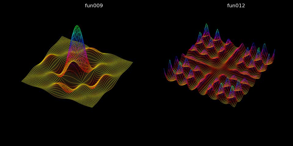
Further examples of viewing line slices are shown below. Line objects were identically constructed as in the previous script with only changes made to the function references.

# 1. Define function to examine .....................................

def fun009(xyz) :
    x,y,z = xyz
    a,b,c = 1,1,15
    lim = 0.001  # use L'Hopital's rule as x -> 0
    A = np.where(np.abs(x)<lim, np.ones(len(x)), np.divide( np.sin(a*x), a*x ) )
    B = np.where(np.abs(y)<lim, np.ones(len(y)), np.divide( np.sin(b*y), b*y ) )
    Z  = c*A*B
    return x,y,Z

def fun012(xyz) :
    x,y,z = xyz
    A = 0.9*np.exp( np.sin(2*x)*np.sin(0.2*y))
    B = 0.9*np.exp( np.sin(2*y)*np.sin(0.2*x))
    Z  = A*B
    return x,y,Z

# 2. Setup and map surfaces .........................................
rez=5
cmap = cmu.hsv_cmap_gradient([1.166,1,1],[0.333,1,1])