Representing f(θ , φ) Contours

This is similar to the surface example Two methods of Representing . The two approaches for coloring contours is also exemplified in Contour Coloring.

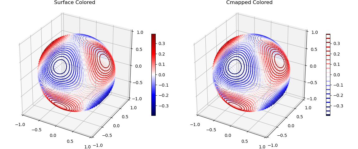
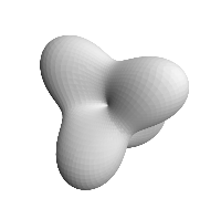
In this example, the primary method of creating contours was to first construct a surface object which is distorted based on the function of interest. For both cases, the spherical object is slightly modified to construct contours, the amount given by expansion variable. The amount of 0.01 is sufficient to create the contours but undetectable in the visualization. Using an exaggerated value for the expansion, the resulting surface object is shown below.

import numpy as np
from scipy import special as sp
from matplotlib import pyplot as plt
from matplotlib.ticker import LinearLocator, FormatStrFormatter
import s3dlib.surface as s3d
import s3dlib.cmap_utilities as cmu

#.. Two methods of Representing f(θ, φ) contours, Real

# 1. Define functions to examine ....................................
expansion = 0.01

def sphHar(rtp) :
    r, theta, phi = rtp
    m, l = 2,3
    r = sp.sph_harm(m, l, theta, phi).real
    return r, theta, phi

def spHar_plusOne(rtp) :
    r, theta, phi = sphHar(rtp)
    return expansion*r+1, theta, phi

def rDir(xyz) : return s3d.SphericalSurface.coor_convert(xyz)[0]

# 2. Setup and map surfaces .........................................
rez = 5
binmap = cmu.binary_cmap()

sph_23 = s3d.SphericalSurface(rez, basetype='octa', cmap='seismic')
sph_23.map_cmap_from_op( lambda rtp : sphHar(rtp)[0] ) 
sph_23.map_geom_from_op(spHar_plusOne) # distortion of sphere to create contours.

surf_contours = sph_23.contourLineSet(20)

temp = sph_23.contourLineSet(20)  # note: temp in xyz coordinates
cmap_contours = temp.map_cmap_from_op(rDir, 'seismic',cname='contour cmap')
cmap_contours.vlim = sph_23.bounds['vlim']  # reset the bounds for the contour cmap

# 3. Construct figure, add surfaces, and plot .....................

fig = plt.figure(figsize=plt.figaspect(0.5/1.2))
ax1 = fig.add_subplot(121, projection='3d', aspect='equal')
ax2 = fig.add_subplot(122, projection='3d', aspect='equal')
ax1.set(xlim=(-1,1), ylim=(-1,1), zlim=(-1,1) )
ax2.set(xlim=(-1,1), ylim=(-1,1), zlim=(-1,1) )
ax1.xaxis.set_major_locator(LinearLocator(5))
ax1.yaxis.set_major_locator(LinearLocator(5))
ax1.zaxis.set_major_locator(LinearLocator(5))
ax2.xaxis.set_major_locator(LinearLocator(5))
ax2.yaxis.set_major_locator(LinearLocator(5))
ax2.zaxis.set_major_locator(LinearLocator(5))
ax1.set_title('Surface Colored')
ax2.set_title('Cmapped Colored')
plt.colorbar(sph_23.cBar_ScalarMappable, ax=ax1,  shrink=0.6 )
plt.colorbar(cmap_contours.stcBar_ScalarMappable(20,'w'), ax=ax2, shrink=0.6 )

ax1.add_collection3d(surf_contours.fade())
ax2.add_collection3d(cmap_contours.fade())

fig.tight_layout(pad=1.5)
plt.show()