Datagrid Geometry

The data used to construct the surface geometry is that used for the Matplotlib Custom hillshading in a 3D surface plot example.

import numpy as np
import matplotlib.pyplot as plt
from matplotlib.ticker import LinearLocator
import s3dlib.surface as s3d
import s3dlib.cmap_utilities as cmu

#.. Matplotlib Examples: Datagrid Geometry

# 1. Define function to examine .....................................

z=np.load('data/jacksboro_fault_dem.npz')['elevation']
datagrid = np.flip( z[5:50, 5:50], 0 )

# 2. Setup and map surfaces .........................................
rez=5
cmu.rgb_cmap_gradient([0.25,0.15,0], [1,.9,.75], 'cardboard' )
ls = s3d.elev_azim_2vector(0,-135)

surface = s3d.PlanarSurface(rez,cmap='cardboard')
surface.map_geom_from_datagrid( datagrid )
surface.map_cmap_from_normals(direction=ls)

# 3. Construct figure, add surface, plot ............................

fig = plt.figure()
fig.text(0.975,0.975,str(surface), ha='right', va='top', fontsize='smaller', multialignment='right')
ax = plt.axes(projection='3d')
ax.set(xlim=(-1,1), ylim=(-1,1), zlim=(0,1) )
ax.xaxis.set_major_locator(LinearLocator(5))
ax.yaxis.set_major_locator(LinearLocator(5))
ax.zaxis.set_major_locator(LinearLocator(6))

ax.add_collection3d(surface)

plt.show()

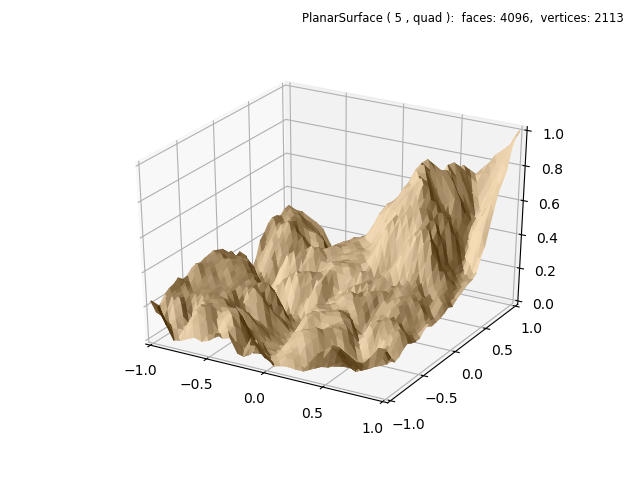
This example uses the datagrid to construct the normalized planar surface. A color map is applied to the face normals to visualize the 3D surface. Note that the array order of the originating datagrid is reversed, shown in the highlighted line, to be consistent with the datagrid coordinate orientation definition. This is further discussed in the Image and Datagrid Mapping guide.

Vertical Colorization

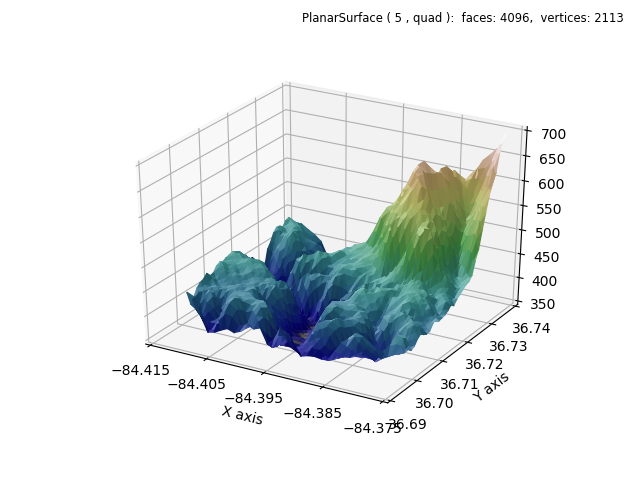
The referenced matplotlib example uses a cmap applied to the vertical location of the surface. This can also be easily constructed since the surface geometry is already applied. A simple lambda function can be used, instead of defining a separate functional operation. The resulting plot is shown below.

import numpy as np
import matplotlib.pyplot as plt
from matplotlib.ticker import LinearLocator
import s3dlib.surface as s3d

#.. Matplotlib Examples: Datagrid Geometry, 2

# 1. Define function to examine .....................................

with np.load('data/jacksboro_fault_dem.npz') as dem :
    z = dem['elevation']
    nrows, ncols = z.shape
    x = np.linspace(dem['xmin'], dem['xmax'], ncols)
    y = np.linspace(dem['ymin'], dem['ymax'], nrows)
    x, y = np.meshgrid(x, y)

region = np.s_[5:50, 5:50]
x, y, z = x[region], y[region], z[region]

datagrid = np.flip(z,0)

# 2. Setup and map surfaces .........................................
rez=5
ls = s3d.elev_azim_2vector(60,180)

surface = s3d.PlanarSurface(rez, cmap='gist_earth')
surface.map_geom_from_datagrid( datagrid )
surface.map_cmap_from_op( lambda xyz : xyz[2] )
surface.shade(0.4,direction=ls).hilite(0.5,direction=ls, focus=0.5)
surface.scale_dataframe(x,y,datagrid)

# 3. Construct figure, add surface, plot ............................

fig = plt.figure()
fig.text(0.975,0.975,str(surface), ha='right', va='top', fontsize='smaller', multialignment='right')
ax = plt.axes(projection='3d')
ax.set(xlim=(-84.415,-84.375), ylim=(36.690,36.740), zlim=(350,700) )
ax.xaxis.set_major_locator(LinearLocator(5))
ax.yaxis.set_major_locator(LinearLocator(6))
ax.zaxis.set_major_locator(LinearLocator(8))
ax.set_xlabel('X axis')
ax.set_ylabel('Y axis')

ax.add_collection3d(surface)

plt.show()

Shading and highlighting are applied to the surface using the light direction shown in the highlighted line. This provided a more direct comparison to the Matplotlib example which uses hillshading. Surface scaling using the dataframe arrays also resized and positioned the surface for displaying data units.