3D Box Surface Plot

Surface geometry is that taken from the matplotlib 3D box surface plot example.

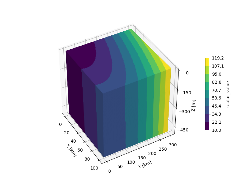
This example uses the predefined cubic surface, with the domain reset from the default domain of [-1,1]. Colors are then directly mapped to the surface object. The Matplotlib example plots line edges to indicate the box edges. As an alternative, the surface was shaded to visualize the 3D surface faces.

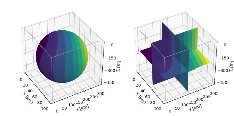
Since the colored cubic surface is composed of all six sides, any orientation can be displayed by simply changing the arguments for the axis view_init method. The color mapping function is applicable throughout the domain allowing interior surfaces of the cube to be colored. Surface examples of this are shown in the following figure, which include lines to indicate box edges.

import numpy as np
import matplotlib.pyplot as plt
from matplotlib import cm,colormaps
from matplotlib.colors import ListedColormap
import s3dlib.surface as s3d

#.. Matplotlib Examples: 3D box surface plot

# 1. Define function to examine ....................................

def scalar_value(xyz) :
    X,Y,Z = xyz
    return  (((X+100)**2 + (Y-20)**2 + 2*Z)/1000+1)

# 2. Setup and map surface .........................................
rez=7
nineColors = ListedColormap( colormaps['viridis'](np.linspace(0, 1, 9)) )

surface = s3d.CubicSurface(rez)
surface.domain( [0,100], [0,300],[-500,0])
surface.map_cmap_from_op(scalar_value,nineColors)
surface.shade(.5,[1,0,2])

# 3. Construct figure, add surface, and plot ......................

fig = plt.figure(figsize=(7.5, 6))
ax = plt.axes(projection='3d', aspect='equal')
ax.set(
    xlabel='X [km]', ylabel='Y [km]', zlabel='Z [m]',
    zticks=[0, -150, -300, -450],
)
ax.view_init(40, -30)
minc, maxc = surface.bounds['vlim']
fig.colorbar(surface.cBar_ScalarMappable, ticks=np.linspace(minc,maxc,10),
    ax=ax, fraction=0.02, pad=0.1, label=surface.cname )

s3d.auto_scale(ax,surface)
ax.add_collection3d(surface)

plt.show()

The additional dataRTP function was added for the spherical surface which uses spherical native coordinates, whereas the data function uses xyz coordinates for color mapping. Also, due to scaled view, the sphere is actually an ellipsoid. Therefore, shading included the argument assignment ax=ax for these cases.

import numpy as np
import matplotlib.pyplot as plt
from matplotlib import cm,colormaps
from matplotlib.colors import ListedColormap
import s3dlib.surface as s3d

#.. Matplotlib Examples: 3D box surface plot, alt example surfaces

# 1. Define function to examine ....................................
def scalar_value(xyz) :
    X,Y,Z = xyz
    return  (((X+100)**2 + (Y-20)**2 + 2*Z)/1000+1)

def dataRTP(rtp) : # note: sphere object uses spherical native coordinates
    return scalar_value( s3d.SphericalSurface.coor_convert(rtp,True) )

# 2. Setup and map surface .........................................
rez=6
nineColors = ListedColormap( colormaps['viridis'](np.linspace(0, 1, 9)) )

sphere = s3d.SphericalSurface(rez)
sphere.transform(scale=[50,150,250],translate=[50,150,-250])
sphere.map_cmap_from_op(dataRTP,nineColors)

plane_z = s3d.PlanarSurface(rez)
plane_y = s3d.PlanarSurface(rez).transform(s3d.eulerRot(0,90))
plane_x = s3d.PlanarSurface(rez).transform(s3d.eulerRot(90,90))
planes = plane_z + plane_y + plane_x
planes.transform(scale=[50,150,250],translate=[50,150,-250])
planes.map_cmap_from_op(scalar_value,nineColors)

surfaces = [ sphere, planes]

#  front edge lines, coordinates/indices
vE = [ [0,0,0], [100,0,0], [100,300,0], [100,0,-500] ]
iE = [ [0,1,2],[1,3]]

# 3. Construct figure, add surface, and plot ......................

fig = plt.figure(figsize=(8, 4))
for i,surface in enumerate(surfaces) :
    ax = fig.add_subplot(121+i, projection='3d', aspect='equal')
    ax.set(
        xlabel='X [km]', ylabel='Y [km]', zlabel='Z [m]',
        zticks=[0, -150, -300, -450],
    )
    ax.view_init(40, -30)
    minc, maxc = surface.bounds['vlim']
    
    s3d.auto_scale(ax,surface)
    ax.add_collection3d(surface.shade(.5,[1,0,2],ax=ax))
    ax.add_collection3d( s3d.ColorLine3DCollection(vE,iE,color='0.6',lw=1) )

fig.tight_layout(pad=2)
plt.show()