Color Mapping Normals

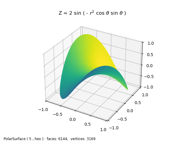
For this example, the surface geometry is similar to that used in the Matplotlib Triangular 3D surfaces example. Using the native coordinates for the PolarSurface object, the mathematical expression is readily seen in the geometric mapping function pringle. Color mapping from the normals provides a 3D effect. For color mapping, default values for the color map and direction are used.

import numpy as np
from matplotlib import pyplot as plt
import s3dlib.surface as s3d
import s3dlib.cmap_utilities as cmu

#.. Matplot: Color Mapping Normals

# 1. Define function to examine .....................................

def pringle(rtz) :
    r,t,z = rtz
    xy = (r**2)*np.cos(t)*np.sin(t)
    Z = 2*np.sin(-xy )
    return r,t,Z

# 2. Setup and map surfaces .........................................

saddle = s3d.PolarSurface(5)
saddle.map_geom_from_op( pringle )
saddle.map_cmap_from_normals()

# 3. Construct figures, add surface, plot ...........................

fig = plt.figure(figsize=plt.figaspect(0.8))
fig.text(0.02,0.02,str(saddle), ha='left', va='bottom', fontsize='smaller')
ax = plt.axes(projection='3d')
minmax, ticks = (-1,1), [-1,-.5,0,.5,1]
ax.set(xlim=minmax,  ylim=minmax,  zlim=minmax,
      xticks=ticks, yticks=ticks, zticks=ticks  )
ax.set_title(r'Z = 2 sin ( - $r^2$ cos $\theta$ sin $\theta$ )')
ax.add_collection3d(saddle)

plt.show()

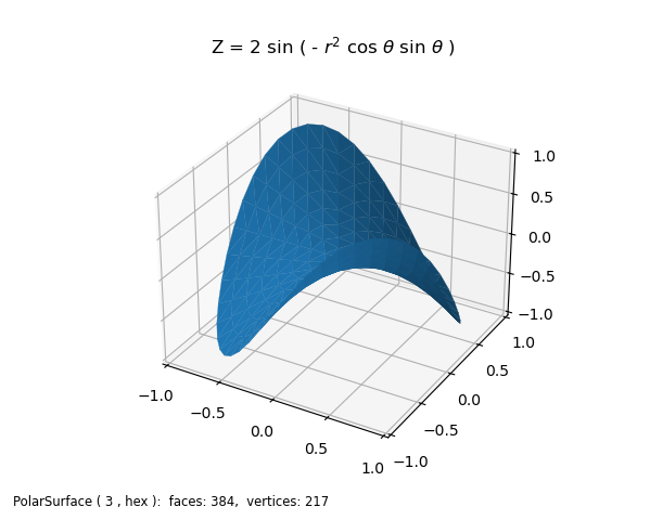
To produce the similar colored view as the Matplolib plot, use shading instead of color mapping normals. This is done by replacing the second section of script by:

# 2. Setup and map surfaces .........................................

saddle = s3d.PolarSurface(3, basetype='hex', linewidth=0.2)
saddle.map_geom_from_op( pringle ).shade(0.3,direction=[-1,-1,1])

which produces the following plot. In this case, a color is not defined in the constructor, so the blue default color is used for the surface color. The edges are visible as a result of setting the linewidth to 0.2, which is further described in the Face and Edge Colors guide.