Iso Cloud

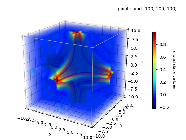
In the Iso Surface and the Alternative Visualizations examples, the ‘mfunc’ is visualized as surfaces evaluated at contant values. Alternatively, using a point cloud allows a 3-D visualization of values within the domain.

import numpy as np
import matplotlib.pyplot as plt
import s3dlib.surface as s3d
import s3dlib.pntcloud as ptc

# 1. Define function to examine .....................................

def mfunc(xyz) :
    x,y,z = xyz
    return np.sin(x*y*z)/(x*y*z)

# 2. Setup and map cloud ............................................
drez, domain = 6.5, 10

cloudObj = ptc.Point3DCloud(drez,cmap='jet',domain=domain)
cloudObj.map_vals_from_op(mfunc)
cloudObj.map_cmap_from_cloudvals()

xlim,ylim,zlim = cloudObj.get_domain()

# 3. Construct figures, add cloud, and plot ........................

fig = plt.figure(figsize=(6.0, 4.5))
fig.text(0.975,0.975,str(cloudObj), ha='right', va='top', fontsize='smaller')
ax = fig.add_subplot(111, projection='3d', aspect='equal', focal_length=0.5)
ax.set(xlim=xlim,ylim=ylim,zlim=zlim,xlabel='x',ylabel='y',zlabel='z')
ax.view_init(20)

cloudObj.add_to3d(ax,1)
s3d.add_boxCorner(ax,domain)

scmp = cloudObj.cBar_ScalarMappable
cbar = plt.colorbar(scmp, ax=ax,  shrink=0.6, pad=.08 )
cbar.set_label('cloud data values', rotation=270, labelpad = 15)

fig.tight_layout(pad=1.5)
plt.show()