Alternative Visualizations

The values of implicit surface functions within a domain are visualized using alternative methods for the function:

f(x,y,z) = sin( x y z ) / ( x y z )

which exhibits Argument Value Sensitivity for anomalous visualizations for various conditions.

Surface Sets

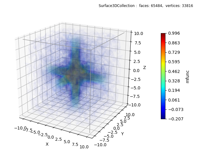
Using multiple semi-transparent contour surfaces provides a visualization of scalar values within a domain.

import numpy as np
import matplotlib.pyplot as plt
import s3dlib.surface as s3d

# 1. Define function to examine ....................................

def mfunc(xyz) :
    x,y,z = xyz
    return np.sin(x*y*z)/(x*y*z)

# 2. Setup and map surface .........................................

surface = s3d.Surface3DCollection.implsurfSet(mfunc,1.9,10,numb=40,cmap='jet')
surface.set_surface_alpha(.015)

# 3. Construct figure, add surface, and plot ......................

fig = plt.figure(figsize=(6.5, 5))
fig.text(0.975,0.975,str(surface), ha='right', va='top', fontsize='smaller')
ax = plt.axes(projection='3d', focal_length=0.5, aspect='equal' )
ax.set(xlabel='X', ylabel='Y', zlabel='Z')
ax.view_init(20)
fig.colorbar(surface.cBar_ScalarMappable, ax=ax, pad=0.1, shrink=0.6,
    ticks=np.linspace(*surface.bounds['vlim'],10), label=surface.cname )
s3d.auto_scale(ax,surface)

ax.add_collection3d(surface.shade(.5))

vE,iE = [ [-10,-10,10], [10,-10,10], [10,10,10], [10,-10,-10] ], [ [0,1,2],[1,3]]
ax.add_collection3d( s3d.ColorLine3DCollection(vE,iE,color='0.6',lw=1) )

fig.tight_layout()
plt.show()

Value Colormapping

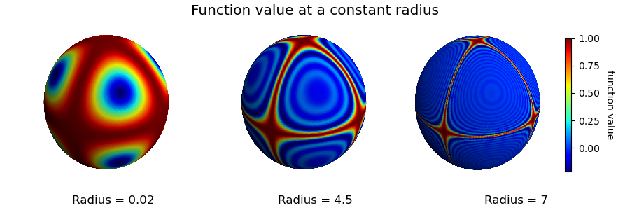
Mapping the values onto spheres illustrates large value fluctuations at larger radial distances from the origin for the cases of small functional values:

import numpy as np
import matplotlib.pyplot as plt
import s3dlib.surface as s3d

# 1. Define function to examine .....................................
def mfunc(xyz) :
    x,y,z = xyz
    return np.sin(x*y*z)/(x*y*z)

val_at_R = lambda rtp : mfunc( s3d.SphericalSurface.coor_convert(rtp,True) )

# 2. Setup and map surfaces .........................................
rez,cmap = 6,'jet'
radius = [.02,4.5,7]
figTitle = 'Function value at a constant radius'
# 3. Construct figure, add surface, plot ............................
ofst = [0.18,0.5,0.82]
fig = plt.figure(figsize=(9,3))
fig.text(0.5,0.98,figTitle, ha='center', va='top', fontsize='x-large')
for i in range(3) :
    title = 'Radius = '+str(radius[i])
    ax =fig.add_subplot(131+i, projection='3d', aspect='equal')
    fig.text(ofst[i],0.02,title, ha='center', va='bottom', fontsize='large')
    ax.set_axis_off()
    surface = s3d.SphericalSurface(rez,cmap=cmap).domain(radius[i])
    surface.map_cmap_from_op( val_at_R )
    usc = .72 if i<=1 else 0.54  # compensate for colorbar space.
    s3d.auto_scale(ax,surface,uscale=1.1*usc)
    ax.add_collection3d(surface.shade())

cbar = plt.colorbar(surface.cBar_ScalarMappable, ax=ax,  shrink=0.7, pad=.1 )
cbar.set_label('function value', rotation=270, labelpad=15)

fig.tight_layout(pad=1)
plt.show()

Geometric and Value Mapping

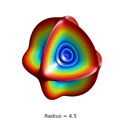
The functional value at a constant radius can be illustrated geometrically by using the value, f, in a multiplier, c, at a radius, R, as:

c(R,θ,φ) = ( 1 + f(R,θ,φ) )

The resulting geometry for a radius of R = 4.5 is :

import numpy as np
import matplotlib.pyplot as plt
import s3dlib.surface as s3d

# 1. Define function to examine .....................................
def mfunc(xyz) :
    x,y,z = xyz
    return np.sin(x*y*z)/(x*y*z)

val_at_R = lambda rtp : mfunc( s3d.SphericalSurface.coor_convert(rtp,True) )

def mod_R(rtp) :
    r,t,p = rtp
    return r*(1 + val_at_R(rtp) ), t, p

# 2. Setup and map surfaces .........................................
rez,R,cmap = 7,4.5,'jet'

surface = s3d.SphericalSurface(rez,cmap=cmap).domain(R)
surface.transform(translate=[0.001,0.001,0.001])  # note: avoid divide by zero.
surface.map_cmap_from_op( val_at_R )
surface.map_geom_from_op (mod_R)

# 3. Construct figure, add surface, plot ............................
fig = plt.figure(figsize=(4,4))
fig.text(.5,0.02,'Radius = '+str(R), ha='center', va='bottom', fontsize='large')
ax = plt.axes(projection='3d', focal_length=0.5, aspect='equal' )
ax.set_axis_off()
s3d.auto_scale(ax,surface,uscale=1.1*(0.72))
ax.add_collection3d(surface.shade().hilite())

fig.tight_layout(pad=0)
plt.show()

Point Cloud

An alternative to visualizing values within the domain is to plot a point cloud of values.

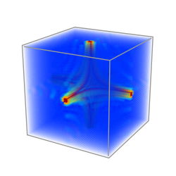
This is shown in the Iso Cloud example.