Argument Value Sensitivity

The effect of increasing rez will generally not affect the overall surface shape visualization other than providing increased detail in the structure. However, when functional values have large fluctuations within local regions of a domain, surface visualizations of constant value become highly dependent on the argument values. The function used in the Iso Surface example exhibit this condition:

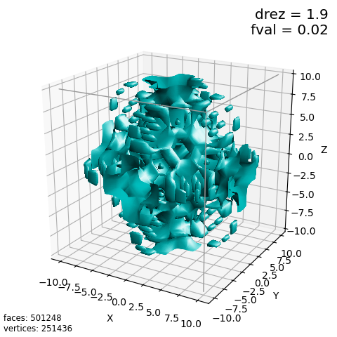
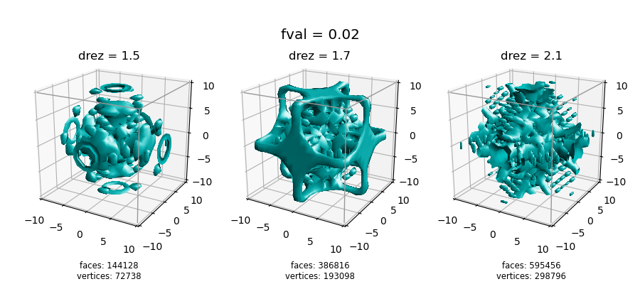
f(x,y,z) = sin( x y z ) / ( x y z )

The above figure shows the surface for constant value of 0.02 using a rez of 1.9. For different value of rez, significantly different visualization result for the same constant, as shown below.

The large fluctuations in functional values near 0.02 can be illustrated using alternative visualizations as shown in the Value Colormapping example.

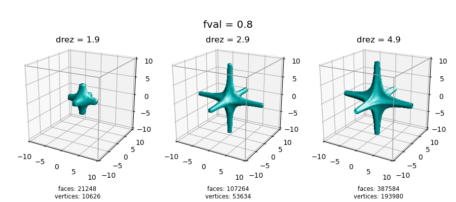
This anomolous surface visualization behavior can be sensitive to the value for the constant. In this functional example, the effect is minimal for larger values as shown below for a value of 0.8. For this constant, increasing rez increases the shape details without significant changes to the overal shape.

The script to generate the first figure is:

import numpy as np
import matplotlib.pyplot as plt
import s3dlib.surface as s3d

# 1. Define function to examine .....................................

def mfunc(xyz) :
    x,y,z = xyz
    return np.sin(x*y*z)/(x*y*z)

# 2. Setup and map surface .........................................
drez,fval=1.9,0.02
surface = s3d.Surface3DCollection.implsurf(mfunc, drez, 10, fval, color='c').evert()
surface.triangulate(3)

# 3. Construct figure, add surface, and plot ......................
ftitle = "drez = "+ str(drez) +"\nfval = " + str(fval)
fig = plt.figure(figsize=plt.figaspect(1))
fig.text(0.975,0.975,ftitle, ha='right', va='top', fontsize='x-large')
info = 'faces: ' + str(len(surface.facecenters.T)) +'\nvertices: ' + str(len(surface.vertices.T))
fig.text(0.01,0.01,info, ha='left', va='bottom', fontsize='smaller')

ax = plt.axes(projection='3d', aspect='equal', focal_length=0.5)
ax.set(xlabel='X',ylabel='Y',zlabel='Z')
ax.view_init(20)
s3d.auto_scale(ax,surface)
surface.shade(0.0,ax=ax,flat=False).hilite(.9,focus=1,flat=False)
ax.add_collection3d(surface)

#  front edge lines, coordinates/indices
vE,iE = [ [-10,-10,10], [10,-10,10], [10,10,10], [10,-10,-10] ], [[0,1,2],[1,3]]
ax.add_collection3d( s3d.ColorLine3DCollection(vE,iE,color='0.6',lw=1) )

fig.tight_layout(pad=2)
plt.show()