Spherical Harmonics Cloud

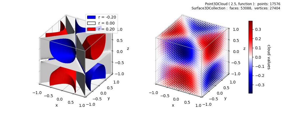
Compared to the Two methods of Representing example, this is an alternative visualization of the 3-D Spherical Harmonics function. The surfaces represent the real values for a constant r within a domain.

import numpy as np
import matplotlib.pyplot as plt
from matplotlib import patches
import s3dlib.surface as s3d
import s3dlib.pntcloud as ptc
from scipy import special as sp

# 1. Define function to examine .....................................

def sphHar(rtp) :
    r, theta, phi = rtp
    m, l = 2,3
    r = sp.sph_harm(m, l, theta, phi).real
    return r, theta, phi

def sphHar_xyz(xyz) :
    rtp = s3d.SphericalSurface.coor_convert(xyz) 
    return sphHar(rtp)[0]

# 2. Setup and map surface .........................................
drez, domain, nsurf, cmap = 2.5, 1, 3, 'seismic'

cloudObj = ptc.Point3DCloud(drez,domain=domain)
cloudObj.map_vals_from_op(sphHar_xyz,cmap)
surface = cloudObj.valsurfSet(nsurf)
surface.triangulate(1)
 
c,v,n =  cloudObj.get_color_for_val( nsurf )
hnd = [patches.Patch(label='r = {:.2f}'.format(v[i]), facecolor=c[i], edgecolor='k' ) for i in range(nsurf) ]
xlim,ylim,zlim = cloudObj.get_domain()

# 3. Construct figures, add surfaces, and plot ....................
fig = plt.figure(figsize=(10,4))
fig.text(.98,.98,str(cloudObj)+'\n'+str(surface),ha='right',va='top', fontsize='smaller')
# ....................
ax = fig.add_subplot(121, projection='3d', aspect='equal',proj_type='ortho')
ax.set(xlim=xlim, ylim=ylim, zlim=zlim, xlabel='x',ylabel='y',zlabel='z')
ax.add_collection3d(surface.shade(ax=ax,flat=False))
s3d.add_boxCorner(ax,domain)
ax.legend(handles=hnd, facecolor='w')
# ....................
ax = fig.add_subplot(122, projection='3d', aspect='equal',proj_type='ortho')
ax.set(xlim=xlim, ylim=ylim, zlim=zlim, xlabel='x',ylabel='y',zlabel='z')
cloudObj.add_to3d(ax)
s3d.add_boxCorner(ax,domain)
# ....................
scmp = cloudObj.cBar_ScalarMappable
cbar = plt.colorbar(scmp, ax=ax,  shrink=0.8, pad=.1 )
cbar.set_label('cloud values', rotation=270, labelpad = 15)
# ....................
fig.tight_layout(pad=3)
plt.show()