Hello World, Lines

This page covers the basics of creating a line plot, introducing the concepts of

• instantiation of a line object
• adding the line object to a 3D axes
• line resolution
• functional mapping

General Concepts

For S3Dlib, a Line is defined as a continuous sequence of linear segments with a common vertex at joining segments (a line can contain a single segment with two vertices).

Throughout this tutorial and all the example plots, the construction and display of lines consist of three basic steps.

1. Define coordinate and coloring, either explicitly or usings functions.
2. Instantiate line objects and apply mapping methods.
3. Setup the Matplotlib figure and axes.

These three steps are similar to those described in the Hello World tutorial for surfaces.

Default 3D Line Collection Base Class

The base class for producing a line object is:

s3d.ColorLine3DCollection(vertexCoor, segmIndices)

This constructor produces a collection of lines or for a single line, the collection is of size one. The vertexCoor is a list (or array-like) of x,y,z coordinates ( list or array of 3 floats). The segmIndices argument is the vertex indices for the lines, which is a N list of lines, each line being a list of M segments.

The following is the script for producing a collection of two lines.

import numpy as np
from matplotlib import pyplot as plt
import s3dlib.surface as s3d

#.. Base Class Line

# 1. Define line to examine .....................................

verts = [ [-1,1,1], [1,1,-1], [1,-1,1] , [0,-1,-1], [-1,0,0]  ]
segin = [ [4,1],[0,2,3] ]         # indices for two lines.
#segin = [ [4,1,0,2,3] ]          # indices for one lines.

# 2. Setup and map line .........................................

lines = s3d.ColorLine3DCollection(verts,segin)

# 3. Construct figure, add line and plot ........................

fig = plt.figure(figsize=plt.figaspect(1))
ax = plt.axes(projection='3d')
ax.set_aspect('equal')
s3d.auto_scale(ax,lines)

ax.add_collection3d(lines)

plt.show()

which produces the following plot:

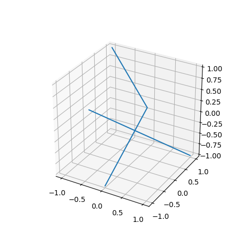
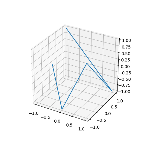
For a single line using the same vertices, only one line is defined in the collection by un-commenting the highlighted code, producing

The line to set the axis limits:

ax.set(xlim=(-1,1), ylim=(-1,1), zlim=(-1,1))

is generally always inserted, over-riding the Matplotlib default axis limits. However, the objects can be used to auto-scale the axes using:

s3d.auto_scale(axes,*obj3d)

where obj3d are the S3Dlib objects, which, for this case is only the line collection object. Auto scaling can often produce plots where the x, y, and z axes are scaled differently. However, using this function can be convenient when the object 3D sizes are unknown prior to plotting.

Single Segmented Line

When a single line object may be constructed from a sequence of vertices, the object can be constructed without the segment indices list. For this case, use:

s3d.SegmentLine(vertexCoor)

A simple example of using just vertex coordinates is that of using a sequence of random walk 3D coordinate locations as shown in the following figure

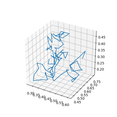
which was produced using the following code. Note that the auto_scale method was used since the range of the result is initially unknown.

import numpy as np
from matplotlib import pyplot as plt
import s3dlib.surface as s3d

#.. Segmented 'continuous' Line

# 1. Define line to examine ......................................

def rand_line(length,seed):
    # Use Matplotlib 'animated 3D random walk' algorithm.
    np.random.seed(seed)
    line_data = np.empty((3, length))
    line_data[:, 0] = np.random.rand(3)
    for index in range(1, length):
        step = (np.random.rand(3) - 0.5) * 0.1
        line_data[:, index] = line_data[:, index - 1] + step
    return line_data.T  #note: transpose

verts = rand_line(100,3)

# 2. Setup and map line ..........................................

line = s3d.SegmentLine(verts)

# 3. Construct figure, add line, and plot ........................

fig = plt.figure(figsize=plt.figaspect(1))
ax = plt.axes(projection='3d')
ax.set_aspect('equal')
s3d.auto_scale(ax,line)

ax.add_collection3d(line)

plt.show()

Parametric Line

A line object with Cartesian coordinates defined by a single parameter is created using the following code:

s3d.ParametricLine(rez,operation)

A ParametricLine object is a sequence of segments, the number be controlled by the rez argument. The operation is the name of a parametric function having one argument in the domain 0 to 1 and returning a set of 3 X N Cartesian coordinates.

Using the rez argument, each segment is recursively subdivided into two segments. The number of recursions (line resolution) is controlled by the rez.

Using the Matplotlib Parametric Curve example, for a rez of 6:

import numpy as np
from matplotlib import pyplot as plt
import s3dlib.surface as s3d

#.. Parametric Line

# 1. Define function to examine .....................................

def parametric_curve(t) :
    #...   0 < t < 1
    r_0, twists = .25, 4
    z = (2*t -1 ) 
    r = r_0 + (1-r_0)*z**2
    theta = twists*np.pi*z
    x = r*np.sin(theta)
    y = r*np.cos(theta)
    return x,y,z

# 2. Setup and map line .............................................
rez=6
line = s3d.ParametricLine(rez,parametric_curve)

# 3. Construct figure, add line, and plot ...........................

fig = plt.figure(figsize=plt.figaspect(1))
ax = plt.axes(projection='3d')
ax.set_aspect('equal')
ax.set(xlim=(-1,1), ylim=(-1,1), zlim= (-1,1) )

ax.add_collection3d(line)

plt.show()

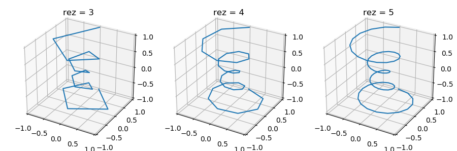
The following figure shows the progressions to higher resolutions for this example of a ParametricLine, from rez=3 to rez=5

Line Fade()

To enhance the line visualization in 3D, a sense of depth for the line can be applied to the line transparency using the line method:

line.fade(depth,elev,azim)

where depth is the minimum color alpha transparency of a line segment, which ranges from 0 to 1. The default value for depth is 0. When applied, the segment alphas will vary from 1 to the set depth aligned from the front to back. Alignment is based on the axis view position set by the elev and azim, in degrees. Then default values are 30 and -60 for elev and azim, respectively.

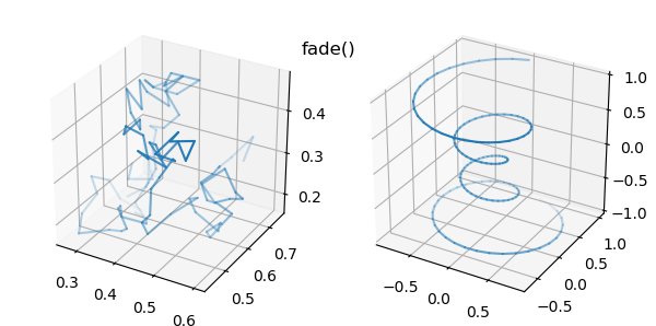
Using the default fade for the previous examples results in the following visualizations of the lines:

Names, Parameterization and Composites

In a similar manner to surface objects, line objects may be added together to form one single ColorLine3DCollection object by simply using the + operator. Also shown in the surface Parametric Functions tutorial, composites object are easily formed by addition, illustrating the parameters controlling the line geometry.

Each of the Line constructors has a named argument ‘name=’, which can also be accessed with setters and getters. As a default, name is an empty string. However, for the ParametricLine object, name will default to the name of the ‘operation’ function, if not a lambda function.

When names are assigned, the axes ‘legend’ will use the line names. The colors displayed in the line legend will be affected by the line shading. When lines are added together to form a composite line, the resulting line has no name until the line name is assigned.

import numpy as np
from matplotlib import pyplot as plt
import matplotlib.patches as mpatches
import s3dlib.surface as s3d

#.. composite versus multiple lines

# 1. Define function to examine .....................................

def parametric_curve(t,N) :
    #...   0 < t < 1
    sc = (2*t -1 )
    r_0, twists = .25, 4
    z = sc 
    r = r_0 + (1-r_0)*z**2
    theta = twists*np.pi*sc
    x = r*np.sin(theta)
    y = r*np.cos(theta)
    return x,y,z + N

def rand_line(length,seed):
    # Use Matplotlib 'Animated 3D Random Walk' algorithm.
    np.random.seed(seed)
    line_data = np.empty((3, length))
    line_data[:, 0] = np.random.rand(3)
    for index in range(1, length):
        step = (np.random.rand(3) - 0.5) * 0.1
        line_data[:, index] = line_data[:, index - 1] + step
    return line_data.T  #note: transpose

verts = lambda s : rand_line(100,s)

fig = plt.figure(figsize=(8,4))

# Axes 1: Parameteric Line composite =======================================
rez=6

line1 = s3d.ParametricLine(rez,lambda t : parametric_curve(t,-.25), color='C0')
line2 = s3d.ParametricLine(rez,lambda t : parametric_curve(t,0.00), color='C1')
line3 = s3d.ParametricLine(rez,lambda t : parametric_curve(t,0.25), color='C2')
line = line1+line2+line3

line.name = "single composite line"
line.shade(0.5).fade(.35)
#.........................
ax1 = fig.add_subplot(121, projection='3d')
ax1.set_aspect('equal')
ax1.set(xlim=(-1,1), ylim=(-1,1), zlim= (-1,1) )
C0_patch = mpatches.Patch(color='C0', label='N = 1')
C1_patch = mpatches.Patch(color='C1', label='N = 2')
C2_patch = mpatches.Patch(color='C2', label='N = 3')
ax1.set_title(line.name)

ax1.add_collection3d(line)  # one line in the collection

ax1.legend(handles=[C0_patch,C1_patch,C2_patch])
# Axes 2 Three Sequence Lines ==========================================

line1 = s3d.SegmentLine(verts(3), color='C0',name='seed: 3')
line2 = s3d.SegmentLine(verts(5), color='C1',name='seed: 5')
line3 = s3d.SegmentLine(verts(6), color='C2',name='seed: 6')
#.........................
ax2 = fig.add_subplot(122, projection='3d')
ax2.set_aspect('equal')
s3d.auto_scale(ax2,line1,line2,line3)
ax2.set_title("three lines")

ax2.add_collection3d(line1)
ax2.add_collection3d(line2)
ax2.add_collection3d(line3)

ax2.legend()
# ===================================================================
fig.tight_layout()
plt.show()

Line Properties

Vertex and segment center coordinates of line objects are accessed using line properties as:

x,y,z = line.vertices

and:

x,y,z = line.segmentcenters

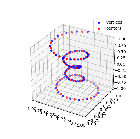
Using the parametric line example, line vertices and segment centers are displayed by using a scatter plot as:

x,y,z = line.vertices
X,Y,Z = line.segmentcenters
ax.scatter(x,y,z,label='vertices',color='b')
ax.scatter(X,Y,Z,label="centers", color='r')
ax.legend()

with the result shown below for a rez of 5.