Hello World

This page covers the basics of creating a surface plot, introducing the concepts of

• instantiation of a surface object
• adding the surface object to a 3D axes
• surface resolution and basetypes
• surface coordinate classes
• functional mapping
• surface properties

General Concepts

Throughout this tutorial and all the example plots, the construction and display of surfaces consist of three basic steps.

1. Define functions for geometric mapping and coloring the surfaces.
2. Instantiate surface objects and apply mapping methods.
3. Set up the Matplotlib figure and axes.

For the first step, all functions controlling geometry and color must accept a coordinate argument of a 3xN Numpy array. The coordinates are in the relative 3D coordinate system. The ‘relative’ system depends on the surface which is to be mapped. These surfaces are in either planar, polar, cylindrical or spherical coordinates.

In the second step, S3Dlib objects are instantiated. All surfaces are defined in normalized coordinates with methods that provide the ability to scale and transform the surface. Surface coordinates are now set using the functions defined in the first step. Also, any colors applied to the surface are made now.

The final step is to use the various tools in Matplotlib to construct and annotate the 3D figure. At the end of this step, the surface objects are simply added to an axes3D as:

axes.add_collection3D(surface)

The addition of the surface to the axes may occur at any step after the axes are created.

Default 3D Surface

The following is the script for producing a default triangulated spherical surface.

import matplotlib.pyplot as plt
import s3dlib.surface as s3d

'''
HELLO WORLD
'''

# Setup surface ................................................

surface = s3d.SphericalSurface()
surface.shade()

# Construct figure, add surface, plot ..........................

fig = plt.figure(figsize=plt.figaspect(1))
ax = plt.axes(projection='3d')
ax.set_aspect('equal')
ax.set(xlim=(-1,1), ylim=(-1,1), zlim=(-1,1))

ax.add_collection3d(surface)

plt.show()

which produces the following plot:

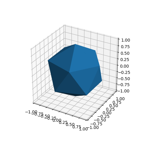
Here, the line:

surface.shade()

is needed to visualize the different faces, otherwise all triangular surfaces would be the same color and only a polygon of uniform color would be recognized. To set the axis limits, use the Matplotlib axis method as:

ax.set(xlim=(-1,1), ylim=(-1,1), zlim=(-1,1))

This is generally always inserted, overriding the Matplotlib default axis limits. Additional methods are available for setting the axis and surface domain as described in the Scaling tutorial.

Surface Resolution

A surface is a collection of polygons that originate by subdividing the base polygons. Each base polygon is recursively subdivided into four subpolygons. The number of recursions (surface resolution) is controlled by the rez, the first argument of the surface constructor. The default rez is 0, as was used in the previous example. This can be explicitly assigned as:

surface = s3d.SphericalSurface(0)

The following figure shows the progressions to higher resolutions for the SphericalSurface, from rez=1 to rez=3

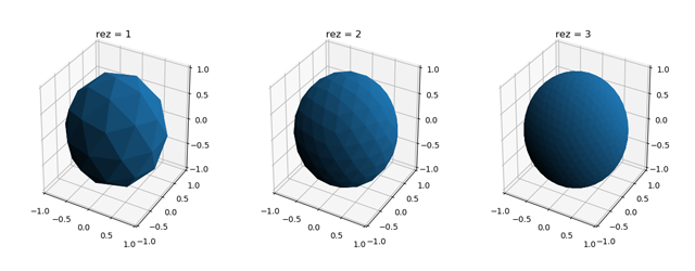
In general, rez is set to a low value, e.g. 2 or 3, during script development for responsive graphic interactivity. Once setup, rez is increased for the desired resolution. A rez of 4 through 6 is sufficient for most surface plots. However, increases to higher rez may be necessary when applying images, using surface clipping or having over-lapping surfaces. This may also be the case for specific geometric mapping functions which produce large surface curvatures.

Basetypes

The SphericalSurface class constructor has the additional argument basetype which is of type string. The basetype sets the initial geometry from which subsequent triangular faces are subdivided using rez values greater than zero. The initial example used the default arguments in the constructor, which can be explicitly set as:

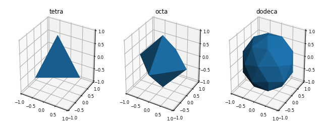
surface = s3d.SphericalSurface(rez=0,basetype='icosa')

The SphericalSurface class has several basetypes based on the Platonic solids. The following figure shows three examples of these basetypes.

Surface Classes

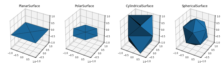
S3Dlib provides several classes to construct a variety of surface objects with associated native coordinate systems. Default objects created with these classes are constructed as:

surfaces[0] = s3d.PlanarSurface()
surfaces[1] = s3d.PolarSurface()
surfaces[2] = s3d.CylindricalSurface()
surfaces[3] = s3d.SphericalSurface()

As with the previous SphericalSurface class example, these constructors have the rez and basetype arguments. The resulting default objects are shown below:

With a variety of classes and basetypes, numerous Base Surfaces can be used for constructing the initial surface objects. Subsequent surface geometry is generated by mapping, as discussed in the next section.

Geometric Mapping

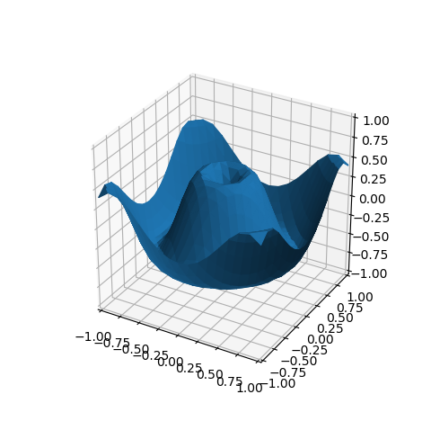
As a starting point, consider the 3D surface example from the Matplotlib gallery. When using S3Dlib, surface coloration and surface geometry are separately applied. Surface coloration is discussed in the subsequent tutorial. For this discussion, the surface color is the default used in the Matplotlib.

The Matplotlib example is in Cartesian coordinates, so a PlanarSurface object will be used for this example instead of the SphericalSurface which was used in the previous example, line 10. First, the function labeled planarfunc is added to the previous script. Then the single highlighted line is added to use this function for mapping the geometry of the planar surface.

Note

Any function definition takes a native coordinate Numpy array argument and returns a Numpy array.

import numpy as np
import matplotlib.pyplot as plt
import s3dlib.surface as s3d

# 1. Define function to examine ....................................

def planarfunc(xyz) :
    x,y,z = xyz
    r = np.sqrt( x**2 + y**2)
    Z = np.sin( 6.0*r )/2
    return x,y,Z

# 2. Setup and map surface .........................................

surface = s3d.PlanarSurface(4)
surface.map_geom_from_op( planarfunc )
surface.shade()

# 3. Construct figure, add surface plot ............................

fig = plt.figure(figsize=plt.figaspect(1))
ax = plt.axes(projection='3d')
ax.set_aspect('equal')
ax.set(xlim=(-1,1), ylim=(-1,1), zlim=(-1,1))

ax.add_collection3d(surface)

plt.show()

Using a rez of 4 produces the following plot.

Surface Properties

Surfaces have accessible properties

• edges
• vertices
• face centers
• face normals
• vertex normals

Edges and face normals are both added to a plot in the similar method used to add the surface object, by using the axes add_collection3d method. Vertices and face centers are coordinate arrays and are added to the figure using the standard Matplotlib 3D scatter plot method, scatter.

The surface object will evaluate as a string to provide information regarding the object class, the rez, and the basetype, along with the number of faces and vertices. For example, for the above object, str(surface) evaluates to the string:

PlanarSurface ( 4 , quad ):  faces: 1024,  vertices: 545

Edges

The edges of the triangulated surface are accessible through an edges property of type ColorLine3DCollection. As a result, this object can be added directly to the axes in a similar manner as the surface object. Instead of adding the surface to the axes, add the edges as:

ax.add_collection3d(surface.edges)

with the result of a wireframe plot as shown below.

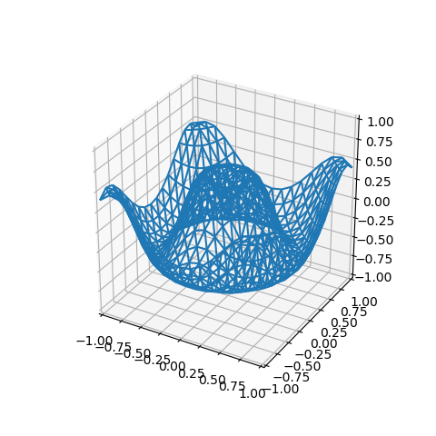
Since the surface faces are not shown, shading may be omitted. Edges of a colored surface will show colors derived from the surface, including shading.

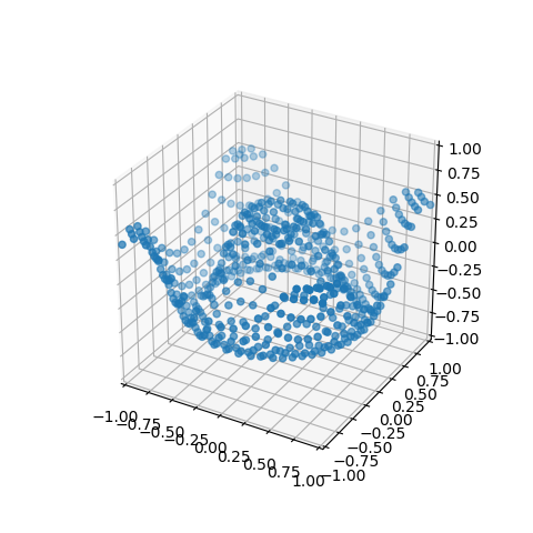
Vertices

The vertices of the triangulated surface are accessible through a surface property of a 3xN coordinate array. These vertices are displayed by creating a simple scatter plot as:

x,y,z = surface.vertices
ax.scatter(x,y,z)

or simply:

ax.scatter(*surface.vertices)

to produce the plot as shown below (the surface is not added to the axes).

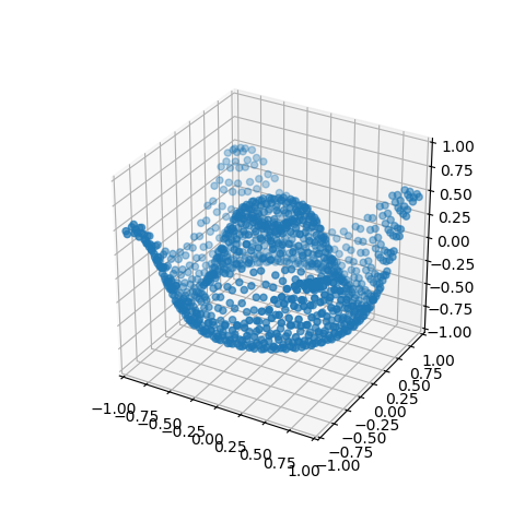
Face Centers

Like the vertices, face centers are a 3xN coordinate array. These face centers are displayed using a scatter plot as:

x,y,z = surface.facecenters
ax.scatter(x,y,z)

or simply:

ax.scatter(*surface.facecenters)

to produce a plot as shown below (the surface is not added to the axes).

Face Normals

Face normals are a Vector3DCollection class which is inherited from the Line3DCollection class. As a result of the inheritance, face normals may be added to the plot similar to adding the surface and edges. The face normals object is accessible from a surface object method. Each normal in the collection corresponds to a face.

These normals are displayed by calling the method and directly passing the result to the axes as:

ax.add_collection3d( surface.facenormals(scale=0.2) )

to produce a plot of vectors as shown below (the surface in not added to the axes). The face normal object properties are controlled using the method arguments which are detailed in the Vector Fields guide. In this example, a scaling factor of 0.2 was used.

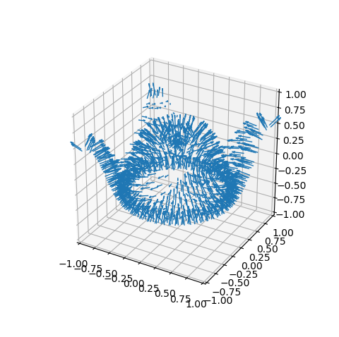
The default color for face normals take the face color, including shading.

Vertex Normals

Vertex normals are a Vector3DCollection class which is inherited from the Line3DCollection class. As a result, vertex normals are added to the plot similar to adding the face normals. Similar to the face normal, added to the axes is:

ax.add_collection3d( surface.vertexnormals(scale=0.2) )

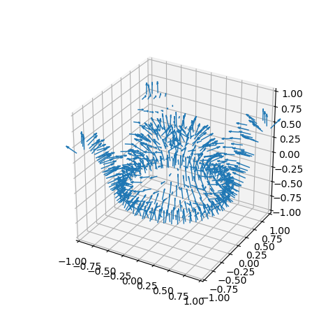
Since normals are associated with the surface resolution, a lower rez is more applicable for visualizing these object properties.

Surface Identifiers

Surface objects have a string representation containing the:

• base class
• rez
• basetype
• number of polygon faces
• number of vertices

For example, the first example surface object represented as a string is obtained using the Python str() method:

str(surface)

which produces:

SphericalSurface ( 0, icosa ): faces:20, vertices:12

In addition, the surface constructors have a name argument which can be used as a specific string identifier. This argument is primarily useful for identifying the surface geometry. The name is an object string property, accessible as:

surface.name

with a default value of a blank string. When the name is not defined in the constructor, the name can also be set by assigning the name argument in the map_geom_from_op method. When no name is assigned in either of these cases, the function argument name is used for the name, provided it is not a lambda expression.

Several colormapping object methods have a cname argument which can be used as string identifier for the coloration. The cname is an object string property, accessible as:

surface.cname

The Hello World Example uses all three of these identifiers to annotate the figure.