Scaling¶

For 3D plotting, the visualization information is not only dependent on the domains of the displayed objects, but the visual ‘form’ of the surfaces which are to be interpreted. The following sections describe the various methods to be applied for displaying 3D objects.

Axis Scaling¶

When Mathplotlib renders a 2D plot, the minimum and maximum for the coordinate axes are automatically set based on the data ranges being plotted. For 3D surfaces, lines, etc., axis scaling cannot generally be relied on for the visualization. As a result, scaling is directly set using these approaches.

explicitly set the axis ranges.
set by axes ranges based on the objects that are added to the 3D axes.
scale all three axes uniformly based on the objects that are added to the 3D axes.

These three approaches are described below.

Explicit Axis Setting¶

The coordinate axes scaling for a 3D plot can be set using the matplotlib.axes.Axes (ax) methods:

ax.set_xlim(left,right)
ax.set_ylim(bottom,top)
ax.set_zlim(bottom,top)

These method have multiple parameters, for example, follow the set_xlim method link.

Most of the examples provided in this S3Dlib documentation use a single method call using named arguments as:

ax.set( xlim=(xmin,xmax), ylim=(ymin,ymax), zlim=(zmin,zmax) )

where a list or tuple of the minimum and maximum values are set for each axis.

Object Axis Setting¶

To exemplify axis scaling based on objects, four surface objects are created and then translated from the origin using the script:

    
    sphere = s3d.SphericalSurface(3,color='r')
    sphere.transform(translate=[0,6,2]).shade()

    icosa = s3d.SphericalSurface(color='b')
    icosa.transform(translate=[-1,1,2]).shade()

    cubeA = s3d.SphericalSurface.platonic(0,'cube_a',color='g')
    cubeA.transform(translate=[0,4,0]).shade()

    cube = s3d.SphericalSurface.platonic(0,'cube',color='y').shade()

Scaling of the axes based on the objects added to the 3D axes, ax, is made using the method:

s3d.auto_scale(ax,*obj3d)

where the first parameter, ax, is the axis object to which 3D objects are added. Multiple object arguments are designated by *obj3d. The result of plotting the four example objects using the auto_scale method is:

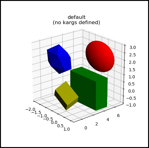
In this case, the ranges for each axis are independently set, based and the maximum and minimum of all objects passed into the auto_scale method as:

s3d.auto_scale(ax,sphere,cube,cubeA,icosa)

where ax is the axes object.

Equal Axis Setting¶

When the set of objects must be viewed with similar scaling along all three coordinate axes, additional named parameters in the the auto_scale method may be passed as:

s3d.auto_scale(ax,*obj3d, **kargs )

key	value when defined	default	control
uscale	float or int	not defined	scale for axis min max limits
rscale	float or int	not defined	scale for axes centered limits

If defined, uscale is a number in the range from 0.5 to 2.5 and is used to scale the range. The default value is 1. Outside of the range, the maximum minimum values will be used. If uscale is not a number, the default value is 1. This provides a simple method of viewing 3D shapes without distortions. So, using a value of True for the four-object example plot:

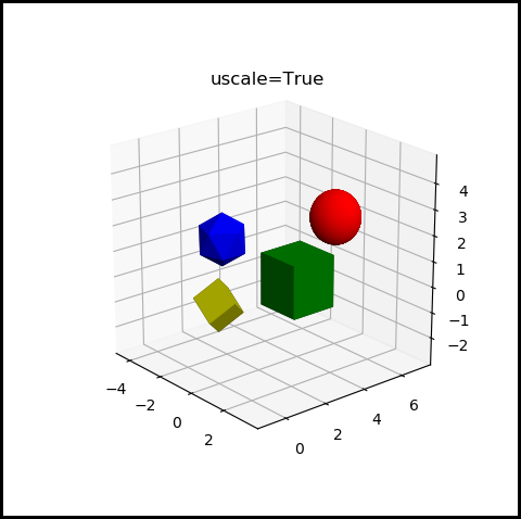
Now spheres, cubes, and icosahedrons appear as spheres, cubes, and icosahedrons without distortion.

In a similar manner, rscale is a scaling factor for axes with min values being the negative of the maximum value. Using rscale produces:

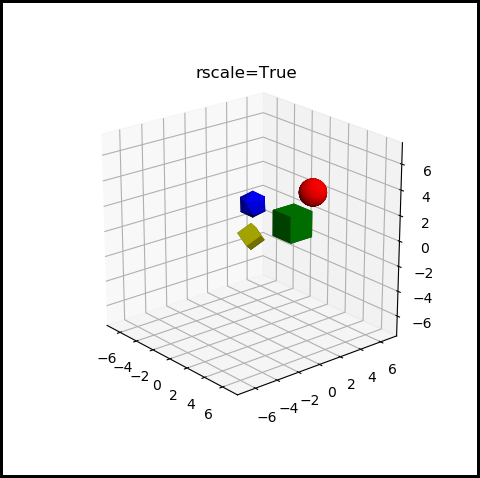
If uscale and rscale are both defined, uscale will be ignored.

Note

The example plots were made with a figure aspect ratio of 1. However, for figures aspects other than 1, the visualizations of these object will be dependent, not only on the axes length ratios, but also the axes viewing elevation and azimuth. Any changes to the elevation or azimuth will change the distortion of the surfaces.

import copy
import numpy as np
import matplotlib.pyplot as plt
import s3dlib.surface as s3d

#.. auto scale demo

# 1. Define functions to examine ....................................
# 2. Setup and map surfaces .........................................

def getObjs() :
    
    sphere = s3d.SphericalSurface(3,color='r')
    sphere.transform(translate=[0,6,2]).shade()

    icosa = s3d.SphericalSurface(color='b')
    icosa.transform(translate=[-1,1,2]).shade()

    cubeA = s3d.SphericalSurface.platonic(0,'cube_a',color='g')
    cubeA.transform(translate=[0,4,0]).shade()

    cube = s3d.SphericalSurface.platonic(0,'cube',color='y').shade()
    
    return sphere,icosa,cubeA,cube

# 3. Construct figure, add surfaces, and plot ......................

# Fig 1 - autoscale,uscale=False (default) -------------------------
fig = plt.figure(figsize=plt.figaspect(1),linewidth=3,edgecolor='k')
fig.tight_layout(pad=0)
ax = plt.axes(projection='3d')
ax.set_aspect('equal')
ax.view_init(22,-40)
ax.set_title('default\n(no kargs defined)')

sphere,cube,cubeA,icosa = getObjs()
ax.add_collection3d(sphere)
ax.add_collection3d(cube)
ax.add_collection3d(cubeA)
ax.add_collection3d(icosa)

s3d.auto_scale(ax,sphere,cube,cubeA,icosa)

# Fig 2 - autoscale,uscale=True ------------------------------------
fig = plt.figure(figsize=plt.figaspect(1),linewidth=3,edgecolor='k')
fig.tight_layout()
ax = plt.axes(projection='3d')
ax.set_aspect('equal')
ax.view_init(22,-40)
ax.set_title('uscale=True')

sphere,cube,cubeA,icosa = getObjs()
ax.add_collection3d(sphere)
ax.add_collection3d(cube)
ax.add_collection3d(cubeA)
ax.add_collection3d(icosa)

s3d.auto_scale(ax,sphere,cube,cubeA,icosa,uscale=True)

# Fig 3 - autoscale,rscale=True ------------------------------------
fig = plt.figure(figsize=plt.figaspect(1),linewidth=3,edgecolor='k')
fig.tight_layout()
ax = plt.axes(projection='3d')
ax.set_aspect('equal')
ax.view_init(22,-40)
ax.set_title('rscale=True')

sphere,cube,cubeA,icosa = getObjs()
ax.add_collection3d(sphere)
ax.add_collection3d(cube)
ax.add_collection3d(cubeA)
ax.add_collection3d(icosa)

s3d.auto_scale(ax,sphere,cube,cubeA,icosa,rscale=True)

# -----------------------------------------------------------------
plt.show()

Shading and Highlighting¶

‘Correct’ shading and highlighting must be viewed with similar scaling along all three axes. When not the case, shading will be ‘distorted’ along with the geometry. To compensate for this effect, the argument ax should be assigned to the 3Daxis for the surface object shade and hilite methods. The following figure shows the effect of axes lengths. The plot on the left shows the ‘actual’ shape of the object. The plot on the right, ‘fits’ the object in scaled axes with scaled shading.

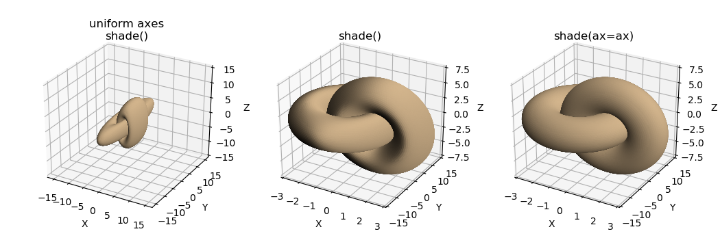
Considering the choices shown in the figure above, the ‘appropriate’ visualization of geometry and shading is dependent on the intention of 3D visualization. Specifically, are X, Y, and Z spatial dimensions or do they represent different dimensional values?

import numpy as np
import copy
from matplotlib import pyplot as plt
import s3dlib.surface as s3d
import s3dlib.cmap_utilities as cmu

#.. Shading : Scaling

# 1. Define function to examine .....................................

def torusFunc(rtz) :
    r,t,z = rtz
    ratio = .5
    Z = ratio*np.sin(z*np.pi)
    R = r + ratio*np.cos(z*np.pi)
    return R,t,Z

# 2. Setup and map surfaces .........................................
a,b,c, pad = 2,10,5, 1.5
posOff, negOff = [0.5,0,0], [-0.5,0,0]
rez = 5

torus_X = s3d.CylindricalSurface(rez,basetype='squ',color='tan' )
torus_X.map_geom_from_op(torusFunc)
torus_X.transform(translate=posOff, rotate=s3d.eulerRot(0,90))
torus_Z = s3d.CylindricalSurface(rez,basetype='squ',color='tan' )
torus_Z.map_geom_from_op(torusFunc)
torus_Z.transform(translate=negOff)

torus = ( torus_X + torus_Z ).transform(scale=[a,b,c])
tori = [ torus, copy.copy(torus), copy.copy(torus) ]

# 3. Construct figure, add surfaces, and plot ......................

A,B,C = pad*a, pad*b, pad*c
title = ['uniform axes\nshade()','shade()','shade(ax=ax)']
fig = plt.figure(figsize=(10.5,3.5))
for i,torus in enumerate(tori) :
    ax = fig.add_subplot(131+i, projection='3d')
    ax.set_aspect('equal')
    ax.set(xlabel='X', ylabel="Y", zlabel="Z" )
    ax.set_title(title[i])
    if i==0 : s3d.auto_scale(ax,torus,uscale=True)
    else :    ax.set(xlim=(-A,A), ylim=(-B,B), zlim=(-C,C))
    links = torus.shade(ax=ax) if i==2 else torus.shade()
    ax.add_collection3d(links)

fig.tight_layout(pad=2)
plt.show()

Object Range¶

The sizes of surface, line and vector objects are determined from the dictionary property bounds. For example, this dictionary for a surface object is:

dict = surface.bounds

The bounds dictionary have values which are 2 element lists for the minimum and maximum values. The keys are shown in the following table:

key	value: [minimum, maximum]
xlim	x range
ylim	y range
zlim	z range
rorg	radial distance from the origin
r_xy	radial distance from the z-axis (xy plane)
vlim	scalar value used for colormapping

Surface Function Domain¶

All base surfaces are initialized in the x,y,z domain from -1 to 1. When plotting 3D functional surfaces, either:

normalize the function of interest into the coordinate domains of -1 to 1, or
change the domain of the base surface prior to functional mapping using the domain method.

For planar base surfaces, domains may be changed using the method:

surface.domain(xlim,ylim,zcoor)

where xlim and ylim are the (min,max) arrays for the x and y domains of the surface. If a single value is used for either xlim or ylim, the domain is set for the plus and minus values. The zcoor is a single z-coordinate value for the plane.

For polar base surfaces, domains may be changed using the method:

surface.domain(radius,zcoor)

where radius is the disk surface radius.

For cylindrical base surfaces, domains may be changed using the method:

surface.domain(radius,zlim)

where zlim is the (min,max) array for the z domain of the surface. If a single value is used for zlim, the domain is set for the plus and minus values.

For spherical base surfaces, domains may be changed using the method:

surface.domain(radius)

For cubic base surfaces, domains may be changed using the method:

surface.domain(xlim,ylim,zlim)

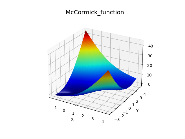
Take for example of the McCormick function which is defined in the domain as:

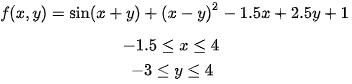
The simple plot, adjusting the domain and using auto scaling is:

import numpy as np
from matplotlib import pyplot as plt
import s3dlib.surface as s3d

# 1. Define function to examine .....................................

def McCormick_function(xyz) :
    x,y,z = xyz
    Z = np.sin(x+y) + (x-y)**2 - 1.5*x + 2.5*y + 1
    return x,y,Z

# 2. Setup and map surfaces .........................................
rez = 6

surface = s3d.PlanarSurface(rez).domain( (-1.5,4.0),(-3.0,4.0) )
surface.map_geom_from_op( McCormick_function )
surface.map_cmap_from_op( lambda C: C[2] , 'jet')

# 3. Construct figure, add surface, plot ............................

fig = plt.figure()
ax = plt.axes(projection='3d')
ax.set_title(surface.name, fontsize='x-large')
ax.set_xlabel('X')
ax.set_ylabel('Y')
s3d.auto_scale(ax,surface)

ax.add_collection3d(surface.shade(.5).hilite(.5))

plt.show()

Table of Contents

Previous topic

Next topic

This Page