3D Rendering

Perceiving 3D objects on a 2D plane requires various visual ‘clues’ in the flat 2D image. Basic options are using lines on the surface object or lightness variations on the surface object. Methods to create such visualizations prior to Matplotlib rendering are:

• distinct edge or line color relative to the face color.
• surface with color mapping in one direction, usually in the vertical z-direction
• surface color shading that is based on surface normals relative to a lighting source position.

The following figure illustrates these three techniques for planar, circumferential and spherical geometries.

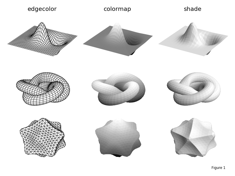
Compared to edge color or color mapping, shading emphasizes the shape for geometries. This is particularly seen in the last example above for the spherical coordinate shape. In addition, s3dlib includes further enhancements to shading for visualizing surfaces and lines. For surfaces, the hilite method can be applied to a shaded surface to provide a ‘glossy’ texture. Highlighting can also enhance the visualization for surfaces with small curvatures. The perception of depth can be applied to lines using the fade method. The following figure illustrates these two methods.

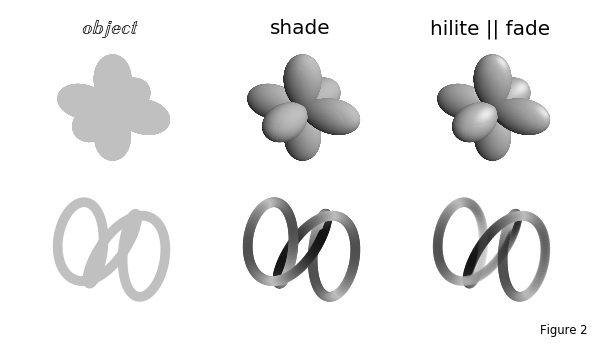
In this above example, the grey colored object is first shown without any applied 3D enhancements prior to rendering. As a result, the three-dimensionality of object is not perceived. The Shading, Highlighting and Color Mapped Normals guide provides detail descriptions of these methods.

For visualizations where portions of the front and back surfaces are viewable, ‘correct’ surface shading is dependent on the orientation of the view. The shade and hilite method have an ax argument that can be assigned to the 3D axis, which accommodates this condition. In addition, use of the axes view with a binary colormap can be used to provide different colors to the front and back surfaces, as shown in the Inner/Outer Surface Colormap example.

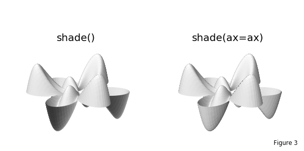
In the above figure, a comparison of shaded visualizations is made for such a surface view. In this case, the ‘bottom’ of the surface turns upward toward the view direction. The left figure only uses the lighting direction to produce shading (for this case, the default direction). The figure on the right uses the view orientation for shading the surface along with the lighting direction. The Open Surfaces : Shading and Highlighting guide provides more detail for using the shade and hilite arguments.

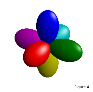
Using shading also provides the additional ability of using color to represent a scalar field or regions on the surface while still emphasizing the shape, as shown in the simple example below:

The approach to shading a surface in Matplotlib differs than that used by S3Dlib. Matplotlib has a LightSource object that may be used with the Axes3D plot_surface method. The S3Dlib shading is a simple ‘KISS’ approach, sufficient for providing the 3D ‘clues’ in the visualization. Differences between S3Dlib and Matplotlib for creating 3D shading ‘clues’ are:

.	S3Dlib	Matplotlib
3D visualization	shade method of an object	LightSource argument of plot_surface
direction specification	Cartesian vectors	elevation and azimuth angles
geometry construction	prior to Axes3D method	during Axes3D method

Using the Cartesian vectors for directions in S3Dlib provides a consistent specification for object orientation, transformations, shading, geometric mapping and color mapping. S3Dlib has two methods, rtv and elev_azim_2vector, to accommodate translating between these two direction descriptions when the axes view_init method is used. Or, as discussed above, the axes argument is provided in the call to the shade and hilite methods. The S3Dlib preference is also based on the intended application, that being a mathematical versus a ‘scene’ perspective.

The S3Dlib ‘geometry construction’ provides a general method of constructing complex 3D visualizations. Although S3Dllib objects are shaded prior to rendering, the advantage of the S3Dlib approach is:

1. A single composite surface can be constructed from multiple objects, preserving the z-order in the single composite. For example Surface Addition, Sub-surface Translation, Composite of Copies.
2. Composite objects can be shaded while retaining individual colormapping of each component. For example Composite Surface of Different Base Surfaces, Angular 4-Color Color Map.
3. Objects can be constructed first, then used to construct other objects. Only the final result needs be rendered. For example Colored Surface Normals, Constant Z Contours of a Function., Mobius From Lines, Spherical Edge Filled Surface.
4. Effects of multiple lighting sources may be applied using combinations of colormapping, shading and highlighting. For example Multiple Lighting, Surface Texture, Inner Glow.
5. Useful for animations, objects can be added and removed from the axes during and after rendering. For example Catenoid to Helicoid, Moon with Rotating Earth. All animations were constructed using this approach for individual frames.

Script code for the above four figures follow:

import copy
import numpy as np
import matplotlib.pyplot as plt
import s3dlib.surface as s3d

# 3D visualizations: edgecolor, colormap, shade

# 1. Define function to examine .....................................
def f_xy(xyz) :
    x,y,z = xyz
    X,Y = 3*x, 3*y
    Z1 = np.exp(-X**2 - Y**2)
    Z2 = np.exp(-(X - 1)**2 - (Y - 1)**2)
    Z = Z1-Z2
    return x,y,Z

def knot(rtz) :
    r,t,z = rtz
    rho,zeta,delta,scale = 0.25, 0.25, 0.3, 0.9
    R = (1-rho)*(1-delta*np.sin(3*t)) + rho*np.cos(z*np.pi) 
    Z = rho*np.sin(z*np.pi) + zeta*np.cos(3*t)
    return scale*R, 2*t, scale*Z

def dimple(rtp) :
    r,t,p = rtp
    depth, delta = 0.2, 0.3
    R = 1-depth*(1-np.cos( (1-r)*np.pi/delta) )
    return R,t,p

def balloon(xyz) :
    r,t,p = s3d.SphericalSurface.coor_convert(xyz,False)
    R = np.power(r,-4)
    return s3d.SphericalSurface.coor_convert([R,t,p],True)

def curl(t) :
    t = 2*np.pi*t
    return np.sin(t), np.cos(3*t), np.sin(3*t)

def petals(rtz) :
    r,t,z = rtz
    minR, N = 0.5, 3
    R = r*( minR + (1-minR)*np.abs(np.cos(N*t)) )
    Z = R*np.cos(N*t)*np.sin(2*np.pi*r)
    return R,t,Z

# FIGURE 1 =================================================================
# 2. Setup and map surf ............................................
rez, nlat,nlng = 4, 18,36

surf = [
    s3d.PlanarSurface(rez,'squ',                 cmap='binary_r',color='w',edgecolor='k',lw=0.5) ,
    s3d.CylindricalSurface.grid(nlat,3*nlng,'r', cmap='binary_r',color='w',edgecolor='k',lw=0.5) ,
    s3d.SphericalSurface.platonic(rez-1,'icosa', cmap='binary',  color='w',edgecolor='k',lw=0.5) 
]
oper = [ f_xy, knot, dimple ]
title = ['edgecolor','colormap','shade']

# 3. Construct figure, add surfaces, and plot ......................
minmax=(-0.85,0.85)
fig = plt.figure(figsize=(8,6))
fig.text(0.9,0.04,'Figure 1', fontsize='small')
for g in range(3) :           #.. geometries
    for t in range(3) :       #.. visualization types
        ax = fig.add_subplot(331+3*g+t,projection='3d') 
        ax.set_aspect('equal')
        ax.set(xlim=minmax, ylim=minmax, zlim=minmax )
        ax.set_axis_off()

        if g == 0 : ax.set_title(title[t],fontsize='x-large')
        surface = copy.copy(surf[g]).map_geom_from_op(oper[g])
        if t == 0 : pass
        if t == 1 : surface.map_cmap_from_op()
        if t == 2 : surface.shade()
        ax.add_collection3d(surface)

fig.tight_layout(h_pad=-4,w_pad=-4)

# FIGURE 2 =================================================================
# 2. Setup and map surf ............................................
rez = 6

obj = [
    s3d.CubicSurface(rez,color='silver').map_geom_from_op(balloon) ,
    s3d.ParametricLine(rez+1,curl,color='silver',lw=7)
]
title = [r'$\mathbb{object}$','shade','hilite || fade']

# 3. Construct figure, add surfaces, and plot ......................
uscale=[0.75,1.1]
fig = plt.figure(figsize=(6,3.5))
fig.text(0.9,0.04,'Figure 2', fontsize='small')
for g in range(2) :           #.. geometries
    for t in range(3) :       #.. visualization types
        ax = fig.add_subplot(231+3*g+t,projection='3d')
        ax.set_axis_off()
        if g == 0 : ax.set_title(title[t],fontsize='x-large')
        sobj = copy.copy(obj[g])
        if t != 0 : sobj.shade()
        if t == 2 :
            if g == 0 : sobj.hilite(0.7,focus=2)
            else :      sobj.fade(.1)
        s3d.auto_scale(ax,sobj,uscale=uscale[g])
        ax.add_collection3d(sobj)

fig.tight_layout(h_pad=-1.7,w_pad=0)


# FIGURE 3 =================================================================
# 2. Setup and map surface .........................................
rez = 4

surface = s3d.PolarSurface.grid(rez*9,rez*36, 'r',color='w')
surface.map_geom_from_op( petals )
surfaces = [ surface, copy.copy(surface)]

# 3. Construct figure, add surface, and plot ......................
fig = plt.figure(figsize=(6,3))
fig.text(0.9,0.04,'Figure 3', fontsize='small')
minmax = (-.8,.8)
for i in range(2) :
    ax =fig.add_subplot(121+i, projection='3d')
    ax.set(xlim=minmax, ylim=minmax, zlim=minmax)
    info = 'shade(ax=ax)' if i==1 else 'shade()'
    ax.set_title('\n\n\n'+info,fontsize='x-large')
    ax.set_axis_off()
    ax.view_init(25,30)
    surface = surfaces[i].shade( ax=ax if i==1 else None)  
    ax.add_collection3d(surface)
fig.tight_layout(pad=0)

# FIGURE 4 =================================================================
# 2. Setup and map surface .........................................
rez=6
colors = ['g','c','m','r','b','y']
surface = s3d.CubicSurface(color=colors).triangulate(rez)
surface.map_geom_from_op(balloon)

# 3. Construct figure, add surface, and plot ......................
fig = plt.figure(figsize=(3, 3))
fig.text(0.8,0.04,'Figure 4', fontsize='small')
ax = plt.axes(projection='3d')
s3d.auto_scale(ax,surface,rscale=0.6).set_axis_off()
ax.set_aspect('equal')
ax.add_collection3d(surface.shade().hilite(0.7,focus=2))

fig.tight_layout()
# ==========================================================================
plt.show()