Complex Number 2D-Representation

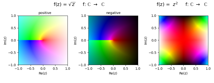
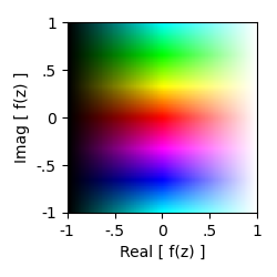
These two complex functions are shown as 3D plots using the z-coordinate color for real and imaginary components in the Complex Number Representation, Geometry and Colormap example. As an alternative, these two components can be shown on 2D plot using the following a Dualcmap:

There are positive and negative solutions for the square root function in Planar Coordinates. As a result, this required subdividing the Dualcmap into two Dualcmaps, as highlighted in the code below. Also, the functional range is normalized in this domain.

import numpy as np
import matplotlib.pyplot as plt
import s3dlib.cmap_utilities as cmu

#.. Complex xy Representation, Dual Colormaps

# custom dualcolormap ....................................

zMap = cmu.hsv_cmap_gradient( [.5,1,1], [1.5,1,1] )
dcmap = cmu.DualCmap('binary_r',zMap,kind='l_y',name='hsv_ly')
posReal = cmu.rgb_cmap_gradient('0.5','1.0')
negReal = cmu.rgb_cmap_gradient('0.0','0.5')
dcmap_p = cmu.DualCmap(posReal,zMap,kind='l_y',name='hsv_ly')
dcmap_n = cmu.DualCmap(negReal,zMap,kind='l_y',name='hsv_ly')

# 1. Define function to examine ....................................

srootp = lambda z :  np.sqrt(z)
srootn = lambda z : -np.sqrt(z)
square = lambda z : z*z

def cmpCmap(x,y,func,cmap) :
    f = func(x+y*1j)
    return cmap(f.real, f.imag).T

# 2. Setup values ........................................
y,x = np.mgrid[ 1:-1:100j,-1:1:100j ]  # note: imshow uses rows, columns

# 3. Construct figure, add surface, and plot ......................
fcc = r'     f: $\mathrm{\mathbb{C}}$ $\to$  $\mathrm{\mathbb{C}}$' +'\n\n'
mmMagDot = [-1,1,-1,1]

fig = plt.figure(figsize=(9,3.5),facecolor='w')
fig.text(0.37,.8,r'f(z) = $\sqrt{z}$' + fcc, fontsize='x-large',ha='center' )
fig.text(0.85,.8,r'f(z) =  $z^2$' + fcc, fontsize='x-large',ha='center' )
fig.text(0.21,.83,'positive',fontsize='medium',ha='center')
fig.text(0.53,.83,'negative',fontsize='medium',ha='center')
# ......................
ax = fig.add_subplot(131, aspect='equal')
ax.imshow(cmpCmap(x,y,srootp,dcmap_p), extent=[*mmMagDot] )
ax.set(xlabel='Re(z)',ylabel=r'Im(z)')
# ......................
ax = fig.add_subplot(132, aspect='equal')
ax.imshow(cmpCmap(x,y,srootn,dcmap_n), extent=[*mmMagDot])
ax.set(xlabel='Re(z)',ylabel=r'Im(z)')
# ......................
ax = fig.add_subplot(133, aspect='equal')
ax.imshow(cmpCmap(x,y,square,dcmap), extent=[*mmMagDot])
ax.set(xlabel='Re(z)',ylabel=r'Im(z)')

fig.tight_layout(pad=1)
plt.show()

Code to plot the Dualcmap is shown below:

import numpy as np
import matplotlib.pyplot as plt
import s3dlib.cmap_utilities as cmu

# custom dualcolormap ....................................
zMap = cmu.hsv_cmap_gradient( [.5,1,1], [1.5,1,1] )
dcmap = cmu.DualCmap('binary_r',zMap,kind='l_y',name='hsv_ly')

y,x = np.mgrid[ 1:-1:100j,-1:1:100j ]  # note: imshow uses rows, columns
mmMagDot,xyticks,xyticklabels = [-1,1,-1,1],[-1,-.5,0,.5,1],['-1','-.5','0','.5','1']

fig = plt.figure(figsize=(2.5,2.5))
ax = plt.axes(aspect='equal')
ax.imshow(dcmap(x,y).T, extent=mmMagDot)
ax.set(xlabel= 'Real [ f(z) ]',ylabel='Imag [ f(z) ]')
ax.set_xticks(xyticks )
ax.set_xticklabels(xyticklabels)
ax.set_yticks(xyticks)
ax.set_yticklabels(xyticklabels)

fig.tight_layout(pad=1)
plt.show()