Dualcmap in Lab Color Space

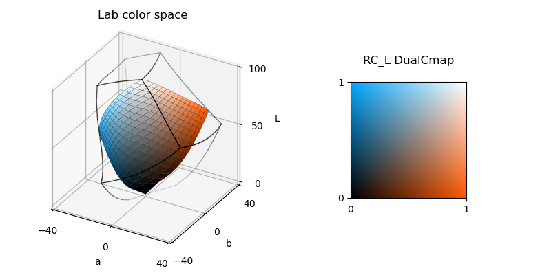
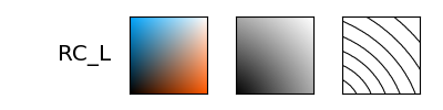
In the above, an example Dualcmap is shown in Lab color space in a similar manner to viewing linear Matplotlib Colormaps in Lab space. Constant L contours can be constructed on the surface, or simply using the show_dualcmaps utility function:

Using the two mapping functions, three basic steps can be used to construct a DualCmap surface in Lab space:

1. Create a PlanarSurface object in the [0,1] xy domain.

2. Map color to the x,y surface coordinates using the Dualcmap.

3. Map the r,g,b colors at the x,y coordinates to lab a,b,L coordinates.

These three steps are highlighted in the following script.

Note

The dualcmap colors are first mapped to a planar grid. As a result, the grid lines in lab space corrospond to contours of constant x or y values in the dualcmap.

import numpy as np
from matplotlib import pyplot as plt
from matplotlib.colors import ListedColormap
from mpl_toolkits.axes_grid1.inset_locator import zoomed_inset_axes
from colorspacious import cspace_converter
import s3dlib.surface as s3d
import s3dlib.cmap_utilities as cmu
import s3dlib.cmap_xtra as cmx

#.. DualCmap in Lab Color Space

# 1. Define function to examine ....................................

def rgb_to_labCoor(rgb):  # X, Y, Z
    L,a,b = cspace_converter("sRGB1", "CAM02-UCS"  )(rgb.T).T
    return a,b,L

def dcmap_to_lab(xyz,dcmap):
    x,y,z = xyz
    rgb = dcmap(x,y)[0:3,:]  # don't include alpha channel
    return rgb_to_labCoor(rgb)

# 2. Setup and map surface .........................................
R = cmu.rgb_cmap_gradient('k',[1.0,0.35,0.0])
C = cmu.rgb_cmap_gradient('k',[0.0,0.65,1.0])
dcmap = cmu.DualCmap(R,C,name='RC_L')   # DualCmap to examine

surface = s3d.PlanarSurface(3,'squ',lw=.15).domain([0,1],[0,1])
surface.map_color_from_op( lambda c: dcmap(c[0],c[1]) ).set_edgecolor('k')
surface.map_geom_from_op( lambda c: dcmap_to_lab(c,dcmap) )

cube = s3d.CubicSurface(color='k').domain([0,1],[0,1],[0,1])
lab_edge = cube.edges.shred(3)
lab_edge.map_geom_from_op(rgb_to_labCoor).set_linewidth(1)

# 3. Construct figure, add surface plot ............................
fig = plt.figure(figsize=(8,4))
ax = fig.add_subplot(121, projection='3d', aspect='equal',proj_type='ortho')
ax.set(xlim=(-40,40), ylim=(-40,40), zlim=(0,100),
    xticks=[-40,0,40],yticks=[-40,0,40],zticks=[0,50,100],
    title='Lab color space', xlabel='a',ylabel='b',zlabel='L')

ax.add_collection3d(surface)
ax.add_collection3d(lab_edge.fade())

#......
ax = fig.add_subplot(122, aspect='equal')
ax.set_axis_off()
ax = zoomed_inset_axes(ax, zoom=-0.5, loc='center')
ax.set(title=dcmap.name+' DualCmap\n ',xticks=[0,1],yticks=[0,1])
y,x = np.mgrid[ 3:-3:100j,-3:3:300j ]  # note: imshow uses rows, columns
ax.imshow(dcmap(x,y).T, extent=[0,1,0,1])

fig.tight_layout(pad=2)

cmx.show_dualcmaps(plt,[dcmap],False)

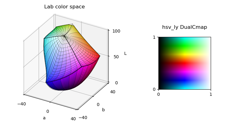
Alternative dualcmaps can be visualized by changing the assignment for dcmap in the above script. For example:

zMap = cmu.hsv_cmap_gradient( [.5,1,1], [1.5,1,1] )
dcmap = cmu.DualCmap('binary_r',zMap,kind='l_y',name='hsv_ly')

produces the following figure (note, the rez was changed from 3 to 4) :