Vector Magnitude/Direction Distribution

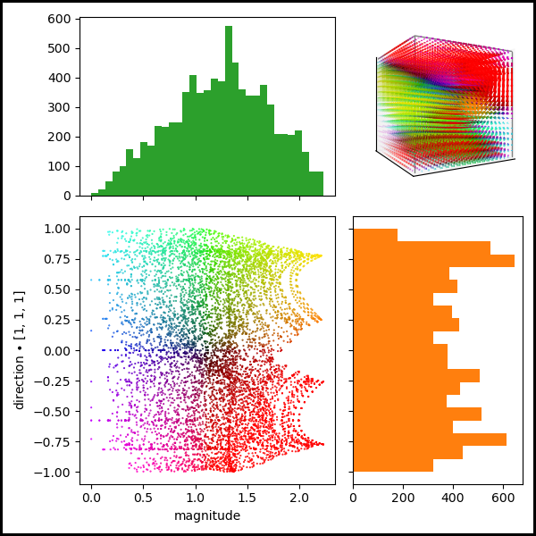
Using the vector field from the previous example, marginal distributions of a scatter plot are shown as histograms at the sides of the plot.

import numpy as np
import matplotlib.pyplot as plt
import s3dlib.surface as s3d
import s3dlib.cmap_utilities as cmu

# Distribution of Vector magnitude and direction

# custom dualcolormap ....................................
kr = cmu.hsv_cmap_gradient( [0.00,1,0], [0.00,1,1], name='black_red' )
kg = cmu.hsv_cmap_gradient( [0.33,1,0], [0.33,1,1], name='black_green' )
bk = cmu.hsv_cmap_gradient( [0.67,1,1], [0.67,1,0] )
rk = cmu.hsv_cmap_gradient( [0.00,1,1], [0.00,1,0] )
bkr = cmu.stitch_cmap(bk,kr, name='blue_k_red')
rkg = cmu.stitch_cmap(rk,kg, name='red_k_green')
dcmap = cmu.DualCmap(bkr,rkg,'srt',name='mcyr')

# 1. Define function to examine ....................................
# +----------------------------------------------------------------------------
# |  The following code between the ========= comments was copied DIRECTLY from
# |  https://docs.enthought.com/mayavi/mayavi/mlab.html#visualizing-a-vector-field
# ===================================================== start of copy.
x, y, z = np.mgrid[0:1:20j, 0:1:20j, 0:1:20j]

u =    np.sin(np.pi*x) * np.cos(np.pi*z)
v = -2*np.sin(np.pi*y) * np.cos(2*np.pi*z)
w = np.cos(np.pi*x)*np.sin(np.pi*z) + np.cos(np.pi*y)*np.sin(2*np.pi*z)
# ===================================================== end of copy.
# ..... reshape data to N x 3 ......................
location = np.reshape(np.array( [x,y,z] ).T,(-1,3))
vector = np.reshape(np.array( [u,v,w] ).T,(-1,3))

# 2. Setup and map vectors ........................................
scale,direction = 0.04, [1,1,1]

vf = s3d.Vector3DCollection(location,scale*vector,alr=0.2)
magdir = [ vf.vectormagnitude/scale, vf.vectordot(direction) ]
vf.map_color_from_op(lambda a,b : dcmap(*magdir))

vE,iE = [ [0,1,1], [0,0,1], [1,0,1], [0,0,0], [1,0,0] ], [ [0,1,2],[1,3],[2,4]]

# Construct figure, add surface & plots ........................
fig, axs = plt.subplots(ncols=2, nrows=2, figsize=(6,6),
        width_ratios=[.6,.4], height_ratios=[.4,.6],
        layout="constrained",linewidth=3,edgecolor='k')
ax = axs[1, 0]              # ... scatter plot
ax.scatter(*magdir,s=1,marker='.',c=vf.vectorcolors)
ax.set(xlabel='magnitude', ylabel=r'direction $\bullet$ '+str(direction))
ax = axs[0, 0]              # ... magnitude histogram
ax.xaxis.set_tick_params(labelbottom=False)
ax.hist(magdir[0], bins='auto', color='tab:green')
ax = axs[1, 1]              # ... direction-dot histogram
ax.yaxis.set_tick_params(labelleft=False)
ax.hist(magdir[1], bins='auto', color='tab:orange', orientation='horizontal')
axs[0,1].set_axis_off()     # ... hide 2D axis, add 3D axis
ax = fig.add_subplot(2,2,2, projection='3d', aspect='equal', focal_length=0.25)
ax.view_init(0,-120)
ax.set(xticks=[], yticks=[], zticks=[] )  
ax.add_collection3d(vf.fade())
ax.add_collection3d( s3d.ColorLine3DCollection(vE,iE,color='0.5',lw=1) )

fig.tight_layout()
plt.show()