Vector DualCmap

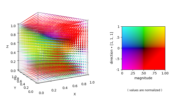
In this example, a vector field is colormapped to to distiguish between the vector magnitude and the direction (referenced using a dot product to a vector.

Additional visualizations of this vector field are given in the Magnitude and Direction Visualization and Vector Surfaces examples.

import numpy as np
import matplotlib.pyplot as plt
import s3dlib.surface as s3d
import s3dlib.cmap_utilities as cmu
from mpl_toolkits.axes_grid1.inset_locator import zoomed_inset_axes

#.. Vector Field Representation, Dual Colormaps

# custom DualCmap ....................................
kr = cmu.hsv_cmap_gradient( [0.00,1,0], [0.00,1,1], name='black_red' )
kg = cmu.hsv_cmap_gradient( [0.33,1,0], [0.33,1,1], name='black_green' )
bk = cmu.hsv_cmap_gradient( [0.67,1,1], [0.67,1,0] )
rk = cmu.hsv_cmap_gradient( [0.00,1,1], [0.00,1,0] )
bkr = cmu.stitch_cmap(bk,kr, name='blue_k_red')
rkg = cmu.stitch_cmap(rk,kg, name='red_k_green')
dcmap = cmu.DualCmap(bkr,rkg,'srt',name='mcyr')

# 1. Define function to examine ....................................
# +----------------------------------------------------------------------------
# |  The following code between the ========= comments was copied DIRECTLY from
# |  https://docs.enthought.com/mayavi/mayavi/mlab.html#visualizing-a-vector-field
# ===================================================== start of copy.
x, y, z = np.mgrid[0:1:20j, 0:1:20j, 0:1:20j]

u =    np.sin(np.pi*x) * np.cos(np.pi*z)
v = -2*np.sin(np.pi*y) * np.cos(2*np.pi*z)
w = np.cos(np.pi*x)*np.sin(np.pi*z) + np.cos(np.pi*y)*np.sin(2*np.pi*z)
# ===================================================== end of copy.
# ..... reshape data to N x 3 ......................
location = np.reshape(np.array( [x,y,z] ).T,(-1,3))
vector = np.reshape(np.array( [u,v,w] ).T,(-1,3))

# 2. Setup and map vectors ........................................
scale,direction = 0.04, [1,1,1]

vf = s3d.Vector3DCollection(location,scale*vector,alr=0.2)
magdir = [ vf.vectormagnitude/scale, vf.vectordot(direction) ]
vf.map_color_from_op(lambda a,b : dcmap(*magdir))

vE,iE = [ [0,1,1], [0,0,1], [1,0,1], [0,0,0], [1,0,0] ], [ [0,1,2],[1,3],[2,4]]

# 3. Construct figure, add vectors, and plot ......................
mag,dotdir = magdir
mmMagDot = [0,1,0,1]
xyticks = [0,0.25,.5,0.75,1]
fig = plt.figure(figsize=(8,4),facecolor='w')
fig.text(0.75,.05,'( values are normalized )',fontsize='small',ha='center')
# ........................
ax = fig.add_subplot(121, projection='3d', aspect='equal', focal_length=0.25)
ax.view_init(0,-120)
ax.set(xlabel='X', ylabel='Y', zlabel='Z' )    
ax.add_collection3d(vf.fade())
ax.add_collection3d( s3d.ColorLine3DCollection(vE,iE,color='0.5',lw=1) )
# ........................
ax = fig.add_subplot(122, aspect='equal')
ax.set_axis_off()
axins = zoomed_inset_axes(ax, zoom=-0.5, loc='center')
y,x = np.mgrid[ 1:0:100j,0:1:100j ]
axins.imshow(dcmap(x,y).T,  extent=[*mmMagDot])
axins.set(aspect='equal')
axins.set(xlabel='magnitude',ylabel=r'direction $\bullet$ '+str(direction))
axins.set_xticks(xyticks)
axins.set_xticklabels(['0','.25','.50','.75','1.00'])
axins.set_yticks(xyticks)
axins.set_yticklabels(['-1','-.5', '0','.5', '1'])

fig.tight_layout(pad=1.5)
plt.show()