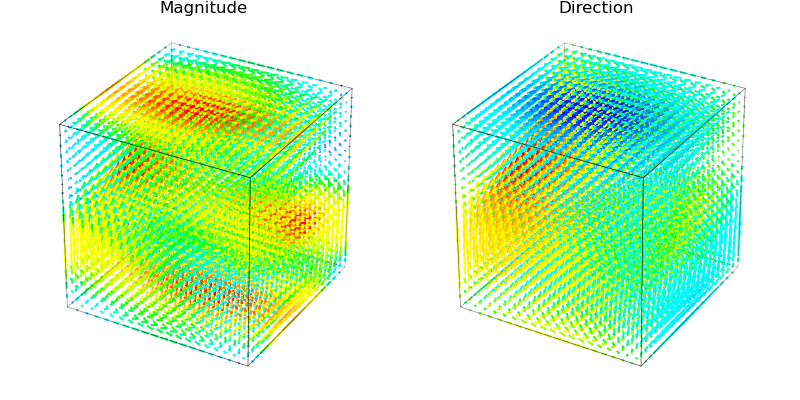
Magnitude and Direction Visualization

The functional description is found at Mayavi vector field example. For the case of dense vector field visualizations, the head and tail of the individual vectors may be difficult to distinguish. For this case, two companion plots can be used to make the distinction.

For this case, the direction value is the dot product with the default direction of [1,1,1].

import numpy as np
from matplotlib import pyplot as plt
import s3dlib.surface as s3d
import s3dlib.cmap_utilities as cmu

# 1. Define function to examine ....................................
# +----------------------------------------------------------------------------
# |  The following code between the ========= comments was copied DIRECTLY from
# |  https://docs.enthought.com/mayavi/mayavi/mlab.html#visualizing-a-vector-field
# ===================================================== start of copy.
x, y, z = np.mgrid[0:1:20j, 0:1:20j, 0:1:20j]

u =    np.sin(np.pi*x) * np.cos(np.pi*z)
v = -2*np.sin(np.pi*y) * np.cos(2*np.pi*z)
w = np.cos(np.pi*x)*np.sin(np.pi*z) + np.cos(np.pi*y)*np.sin(2*np.pi*z)
# ===================================================== end of copy.

# ..... reshape data to N x 3 ......................
scale = 0.04
location = np.reshape(np.array( [x,y,z] ).T,(-1,3))
vector = np.reshape(np.array( [u,v,w] ).T,(-1,3))
vector *= scale

# 2. Setup and map vectors ........................................
cmap = cmu.hue_cmap('b','r',2.0,name='BlRd')

vf_m = s3d.Vector3DCollection(location,vector,alr=0.2)
vf_m.map_cmap_from_magnitude(cmap)

vf_d = s3d.Vector3DCollection(location,vector,alr=0.2)
vf_d.map_cmap_from_direction(cmap)

# 3. Construct figure, add surface, and plot ......................

fig = plt.figure(figsize=(8,4),facecolor='w')
minmax, axPos = (0,1), 121
for vf in [ vf_m,vf_d ] :
    box = s3d.CubicSurface(color='k').domain([0,1],[0,1],[0,1]).edges
    box.set_color('k')
    box.set_linewidth(0.5)
    ax = fig.add_subplot(axPos, projection='3d', aspect='equal', focal_length=0.25)
    ax.view_init(0,-120)
    ax.set(xlim=minmax, ylim=minmax, zlim=minmax,
        xlabel='X', ylabel='Y', zlabel='Z' )
    ax.set_title(vf.cname,fontsize='large')
    axPos += 1

    ax.add_collection3d(vf)
    ax.add_collection3d(box)

fig.tight_layout(pad=2)
plt.show()

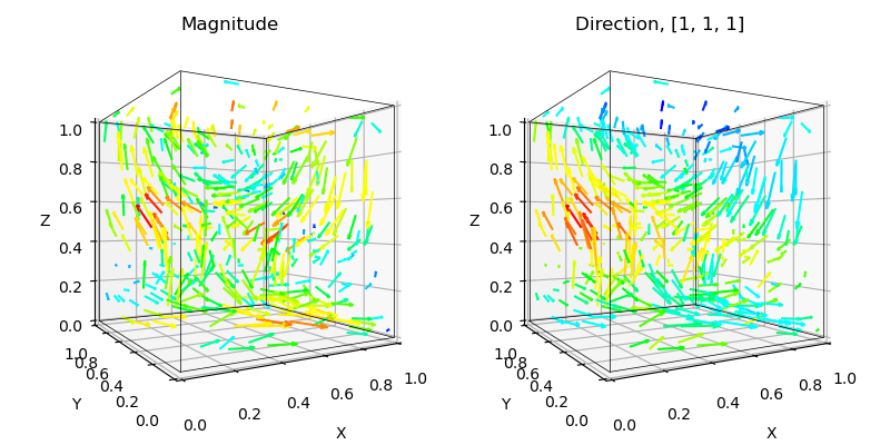
The field is more apparent for a less dense visualization, by evaluating only 1 out of 20 xyz-coordinates:

np.random.seed(1)
N = 400  #  ie.    1 out of 20: (20*20*20)/20
x = np.random.uniform(0, 1, N)
y = np.random.uniform(0, 1, N)
z = np.random.uniform(0, 1, N)

and setting the scale = 0.1, the resulting figure is:

Interpreting this field as surfaces is shown in the Vector Surfaces example.