(x,y) Dataset Density 2

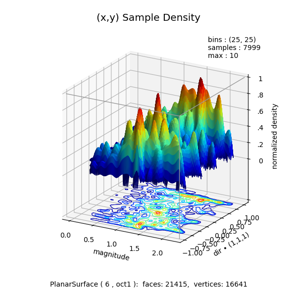
This example demonstrates a 3D data density visualization. A detailed dataset was generated based on the Vector DualCmap vector field distribution, as shown in the Vector Magnitude/Direction Distribution example.

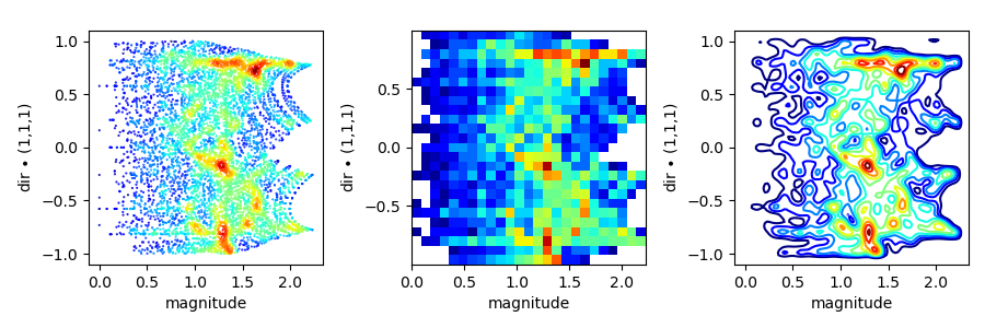
The 2D plots using the Matplotlib axis functions are shown below.

import numpy as np
import matplotlib.pyplot as plt
from matplotlib import cm,colormaps,colors
import s3dlib.surface as s3d

# 1. Define function to examine .......................................

x, y, z = np.mgrid[0:1:20j, 0:1:20j, 0:1:20j]
u =    np.sin(np.pi*x) * np.cos(np.pi*z)
v = -2*np.sin(np.pi*y) * np.cos(2*np.pi*z)
w = np.cos(np.pi*x)*np.sin(np.pi*z) + np.cos(np.pi*y)*np.sin(2*np.pi*z)
location = np.reshape(np.array( [x,y,z] ).T,(-1,3))
vector = np.reshape(np.array( [u,v,w] ).T,(-1,3))
scale,direction = 0.04, [1,1,1]
vf = s3d.Vector3DCollection(location,scale*vector,alr=0.2)
magdir = [ vf.vectormagnitude/scale, vf.vectordot(direction) ]
data = np.array(magdir)
xlbl,ylbl = 'magnitude', r'dir $\bullet$ (1,1,1)'

# .....................................................................
bns  = (25,25)
f,dndmn = s3d.density_function(data,bns, False)    # returns density = f(x,y) & domain

def expand_xyDomain(dmn,scale=1) :
    xmin,xmax,ymin,ymax,__,__ = dmn.flatten()
    xmid,ymid = (xmax+xmin)/2 , (ymax+ymin)/2
    xrng,yrng = (xmax-xmin) , (ymax-ymin)
    xminxmax = [xmid-scale*xrng/2, xmid+scale*xrng/2]
    yminymax = [ymid-scale*yrng/2, ymid+scale*yrng/2]
    return [ xminxmax,yminymax ]

surfDist = lambda c : [c[0],c[1],f(c[0],c[1])]

# 2. Setup and map surfaces .........................................
rez,cmap,domain = 6, colormaps['jet'] , expand_xyDomain(dndmn,1.1)

surface = s3d.PlanarSurface(rez,'oct1',cmap=cmap).domain(*domain)
surface.map_geom_from_op(surfDist)
surface.clip( lambda c: c[2] > 1 )         # clip empty bins
zmax = surface.bounds['zlim'] [1]
surface.transform(scale=[1,1,1/zmax])      # normalize to maximum value
surface.map_cmap_from_op(lambda c: c[2])

zoffset = -1/2                             # contour viewing z-plane
contours = surface.contourLineSet(8)
contours.set_linewidth(0.75)
contours.map_to_plane(zoffset)

# FIGURE 1 : Sample Density Surface ============================================
# ==============================================================================
# 3. Construct figure, add surface, plot ............................

xlim,ylim,zlim = domain + [[zoffset,1.0]]
zticks = [zoffset,0,.2,.4,.6,.8,1]
ztl = ['','0','.2','.4','.6','.8','1']

fig = plt.figure(figsize=(6,6))
info = 'bins : {}\nsamples : {}\nmax : {}'.format(bns,len(data[0]),int(zmax))
fig.text(.5,.94,"(x,y) Sample Density", va='center',ha='center', fontsize='x-large' )
fig.text(.7,.8,info,va='bottom',ha='left')
fig.text(.5,.03,str(surface),va='bottom',ha='center')

ax = plt.axes(projection='3d', aspect='equal',proj_type='ortho')
ax.set(xlabel=xlbl,ylabel=ylbl,zlabel='normalized density',
    xlim=xlim,ylim=ylim,zlim=zlim,
    zticks=zticks,zticklabels=ztl)
ax.view_init(20)
ax.add_collection3d(contours)
ax.add_collection3d(surface.shade())
s3d.add_boxCorner(ax,[xlim,ylim,zlim])

# FIGURE 2 : Data plot, 2D histogram, contours =================================
# ==============================================================================
# 3. Construct figure, 2D plots ............................

fig = plt.figure(figsize=(9,3))
#..................................................... samples x,y plot
ax = fig.add_subplot(131)
ax.set( xlabel=xlbl,ylabel=ylbl)
ax.set_box_aspect(1)
ax.scatter(*data,c=f(*data),s=1,marker='.',cmap=cmap)
#..................................................... density 2D histogram
ax = fig.add_subplot(132)
ax.set( xlabel=xlbl,ylabel=ylbl)
ax.set_box_aspect(1)
w_cmap = cmap(np.linspace(0, 1, 256))
w_cmap[0] = np.array( [1,1,1,1] )  # white = no content.
w_cmap = colors.ListedColormap(w_cmap)
ax.hist2d(*data,bins=bns, cmap=w_cmap)
#..................................................... contour lines
ax = fig.add_subplot(133)
ax.set( xlabel=xlbl,ylabel=ylbl)
ax.set_box_aspect(1)
x,y = np.linspace(*domain[0], 100), np.linspace(*domain[1], 100)
X, Y = np.meshgrid(x, y)
Z = f(X,Y)/zmax                    # normalize for normalized levels
levels = [ i for i in np.arange(.1,1,.1)]
extent=(*domain[0],*domain[0])
lines = ax.contour(X, Y, Z, levels=levels, cmap='jet',origin=None, extent=extent)
#.........................................................
fig.tight_layout()

# ==============================================================================
plt.show()