(x,y) Dataset Density

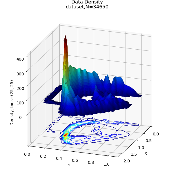
This example demonstrates a 3D data density visualization. A detailed dataset was generated based on the swirl surface face characteristics, as shown in the Surface Face Distributions example.

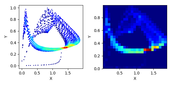
The 2D plots using the Matplotlib axis functions are shown below.

import numpy as np
import matplotlib.pyplot as plt
from matplotlib import cm,colormaps,colors
import s3dlib.surface as s3d

# 1. Define function to examine .......................................

surface = s3d.SphericalSurface.grid(5*20,7*25)
surface.map_geom_from_op(lambda c: [2+np.sin(7*c[1]+5*c[2]),c[1],c[2]] )
data = np.array(surface.area_h2b)
xlbl,ylbl = 'area','h2b'

# .....................................................................
bns  = (25,25)
f,dndmn = s3d.density_function(data,bns, False)    # returns density = f(x,y) & domain

def expand_xyDomain(dmn,scale=1) :
    xmin,xmax,ymin,ymax,__,__ = dmn.flatten()
    xmid,ymid = (xmax+xmin)/2 , (ymax+ymin)/2
    xmid,ymid = (xmax+xmin)/2 , (ymax+ymin)/2
    xrng,yrng = (xmax-xmin) , (ymax-ymin)
    xminxmax = [xmid-scale*xrng/2, xmid+scale*xrng/2]
    yminymax = [ymid-scale*yrng/2, ymid+scale*yrng/2]
    return [ xminxmax,yminymax ]

surfDist = lambda c : [c[0],c[1],f(c[0],c[1])]

# 2. Setup and map surfaces .........................................
rez,cmap,domain = 6, colormaps['jet'] , expand_xyDomain(dndmn,1.1)

surface = s3d.PlanarSurface(rez,'oct1',cmap=cmap).domain(*domain)
surface.map_geom_from_op(surfDist)
surface.clip( lambda c: c[2] > 1 )         # clip empty bins
zmax = surface.bounds['zlim'] [1]
surface.transform(scale=[1,1,1/zmax])      # normalize to maximum value
surface.map_cmap_from_op(lambda c: c[2])

zoffset = -1/2                             # contour viewing z-plane
contours = surface.contourLineSet(10)
contours.set_linewidth(0.75)
contours.map_to_plane(zoffset)

# FIGURE 1 : Sample Density Surface ============================================
# ==============================================================================
# 3. Construct figure, add surface, plot ............................

xlim,ylim,zlim = domain + [[zoffset,1.0]]
zticks = [zoffset,0,.2,.4,.6,.8,1]
ztl = ['','0','.2','.4','.6','.8','1']

fig = plt.figure(figsize=(6,6))
info = 'bins : {}\nsamples : {}\nmax : {}'.format(bns,len(data[0]),int(zmax))
fig.text(.5,.94,"(x,y) Sample Density", va='center',ha='center', fontsize='x-large' )
fig.text(.7,.8,info,va='bottom',ha='left')
fig.text(.5,.03,str(surface),va='bottom',ha='center')

ax = plt.axes(projection='3d', aspect='equal',proj_type='ortho')
ax.set(xlabel=xlbl,ylabel=ylbl,zlabel='normalized density',
    xlim=xlim,ylim=ylim,zlim=zlim,
    zticks=zticks,zticklabels=ztl)
ax.view_init(20)
ax.add_collection3d(contours)
ax.add_collection3d(surface.shade())
s3d.add_boxCorner(ax,[xlim,ylim,zlim])

# FIGURE 2 : Data plot, 2D histogram, contours =================================
# ==============================================================================
# 3. Construct figure, 2D plots ............................

fig = plt.figure(figsize=(9,3))
#..................................................... samples x,y plot
ax = fig.add_subplot(131)
ax.set( xlabel=xlbl,ylabel=ylbl)
ax.set_box_aspect(1)
ax.scatter(*data,c=f(*data),s=1,marker='.',cmap=cmap)
#..................................................... density 2D histogram
ax = fig.add_subplot(132)
ax.set( xlabel=xlbl,ylabel=ylbl)
ax.set_box_aspect(1)
w_cmap = cmap(np.linspace(0, 1, 256))
w_cmap[0] = np.array( [1,1,1,1] )  # white = no content.
w_cmap = colors.ListedColormap(w_cmap)
ax.hist2d(*data,bins=bns, cmap=w_cmap)
#..................................................... contour lines
ax = fig.add_subplot(133)
ax.set( xlabel=xlbl,ylabel=ylbl)
ax.set_box_aspect(1)
x,y = np.linspace(*domain[0], 100), np.linspace(*domain[1], 100)
X, Y = np.meshgrid(x, y)
Z = f(X,Y)/zmax                    # normalize for normalized levels
levels = [ i for i in np.arange(.1,1,.1)]
extent=(*domain[0],*domain[0])
lines = ax.contour(X, Y, Z, levels=levels, cmap='jet',origin=None, extent=extent)
#.........................................................
fig.tight_layout()

# ==============================================================================
plt.show()