Hello World Example 2

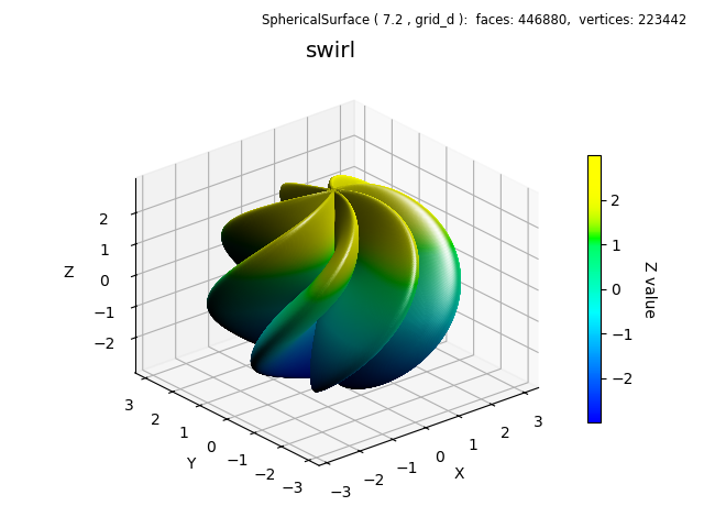
This example adds a few more basic methods which are convenient for function visualization. Highlighted below are for creating custom colormaps, using a grid surface having native spherical coordinates, and auto scaling.

This example uses the function described in the Matlab Parameterized Surface Plot .

import numpy as np
from matplotlib import pyplot as plt
import s3dlib.surface as s3d
import s3dlib.cmap_utilities as cmu

#.. swirl function from
#   https://www.mathworks.com/help/matlab/ref/fsurf.html#bu62pyy-21

# 1. Define function to examine .....................................

def swirl(rtp) :
    r,t,p = rtp
    u,v = t,p
    R = 2 + np.sin(7*u + 5*v)
    return R,t,p

vertical = lambda rtp : s3d.SphericalSurface.coor_convert(rtp,True)[2]
    
# 2. Setup and map surfaces .........................................
b_c = cmu.hue_cmap('b', 0.4, 1.0)
c_y = cmu.hue_cmap(0.4, 'y', 5.0)
b_y = cmu.stitch_cmap(b_c,c_y, bndry=0.66)
mlt = 80
surface = s3d.SphericalSurface.grid(5*mlt,7*mlt,minrad=0.01)
surface.map_geom_from_op( swirl )
surface.map_cmap_from_op( vertical , b_y, cname='Z value' )

# 3. Construct figure, add surface, plot ............................

fig = plt.figure()
fig.text(0.975,0.975,str(surface), ha='right', va='top', fontsize='smaller')
ax = plt.axes(projection='3d')
ax.set_title('\n'+surface.name, fontsize='x-large')
cbar = plt.colorbar(surface.cBar_ScalarMappable, ax=ax,  shrink=0.6 )
cbar.set_label(surface.cname, rotation=270, labelpad = 15)
ax.set( xlabel='X', ylabel='Y', zlabel='Z')
ax.view_init(25,-130)
ax.set_proj_type('ortho')
s3d.auto_scale(ax,surface)

ax.add_collection3d(surface.shade().hilite(direction=[-.4,-1,1],focus=2.5))

fig.tight_layout()
plt.show()

For simple functional relationships, these ‘hello world’ examples only need to be slightly modified. For example:

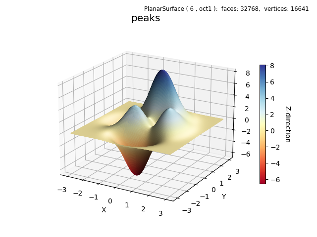
The following includes the use of initializing the surface domain prior to setting the geometry. A default direction for the PlanarSurface object is now used instead of defining a separate function for simple mapping in the z-direction.

This example uses the function described in the Matlab peaks function .

import numpy as np
from matplotlib import pyplot as plt
import s3dlib.surface as s3d

#.. Hello World Example 2, peaks function from
#   https://www.mathworks.com/help/matlab/ref/peaks.html

# 1. Define function to examine .....................................

def peaks(xyz) :
    x,y,z = xyz
    z =  3*(1 - x)**2 * np.exp(-x**2 - (y + 1)**2) \
        - 10*(x/5 - x**3 - y**5)*np.exp(-x**2 - y**2) \
        - 1./3*np.exp(-(x + 1)**2 - y**2) 
    return x,y,z

# 2. Setup and map surfaces .........................................
rez = 6

surface = s3d.PlanarSurface(rez,'oct1',cmap='RdYlBu').domain(3,3)
surface.map_geom_from_op( peaks )
surface.map_cmap_from_op( )

# 3. Construct figure, add surface, plot ............................

fig = plt.figure(figsize=plt.figaspect(0.75))
ax = plt.axes(projection='3d')
ax.view_init(20)
s3d.auto_scale(ax,surface)

fig.text(0.975,0.975,str(surface), ha='right', va='top', fontsize='smaller')
ax.set_title(surface.name, fontsize='x-large')
cbar = plt.colorbar(surface.cBar_ScalarMappable, ax=ax,  shrink=0.6 )
cbar.set_label(surface.cname, rotation=270, labelpad = 15)
ax.set( xlabel='X', ylabel='Y', zlabel='Z')

ax.add_collection3d(surface.shade().hilite(.5))

fig.tight_layout(pad=2)
plt.show()