Alternative Coordinate View

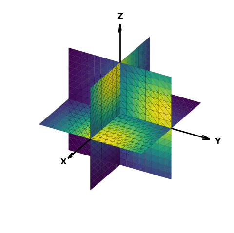
The base surfaces are oriented in the xyz plane with z-coordinate positive upward. This example demonstrates methods for starting with a base plane, then changing the upward direction of the x and y axis of the plane. For the visualization, the three surfaces are combined.

An alternative method of changing xyz coordinates with a function using map_geom_from_op is by rotation with the transform method:

xplane.transform(matrixX)
yplane.transform(matrixY)

which would replace the highlighted lines in the script. Three alternative transform matrix pairs can be constructed using Euler angles as:

matrixX = s3d.eulerRot( 90, 90,useXconv=True )
matrixY = s3d.eulerRot(-90,-90,useXconv=False)

or by setting the directions of the new axis directions as:

matrixX = s3d.vectRot([0,1,0],[0,0,1])
matrixY = s3d.vectRot([0,0,1],[1,0,0])

or by rotation about the [1,1,1] direction as:

matrixX = s3d.axisRot(-120,[1,1,1]))
matrixY = s3d.axisRot( 120,[1,1,1]))

Use of either of these matrix pairs will produce the same visualization.

import copy
import numpy as np
import matplotlib.pyplot as plt
import s3dlib.surface as s3d

#.. PlanarSurface base class viewed in alternative coordinate planes.

# 1. Define function to examine ....................................

X_plane = lambda c : [ c[1],c[2],c[0] ]
Y_plane = lambda c : [ c[2],c[0],c[1] ]

ofsetRad = lambda c : np.exp( -( (c[0]-0.85)**2 + (c[1]-0.25)**2 ) )

# 2. Setup and map surface .........................................
rez = 3

zplane = s3d.PlanarSurface( rez,'oct1').map_cmap_from_op(ofsetRad)
xplane = copy.copy(zplane)
xplane.map_geom_from_op(X_plane)
yplane = copy.copy(zplane)
yplane.map_geom_from_op(Y_plane)

planes = xplane + yplane + zplane
planes.set_edgecolor('k')
planes.set_linewidth(0.1)

# 3. Construct figure, add surface, and plot ......................

fig = plt.figure(figsize=plt.figaspect(1))
ax = plt.axes(projection='3d', aspect='equal')
ax.set_proj_type('ortho')
ax.set( xlabel='X', ylabel='Y', zlabel='Z', )
s3d.standardAxis(ax,offset=1,length=1.75,alr=0.2)
planes.shade(.5)
planes.set_edgecolor('k')
planes.set_linewidth(0.1)
s3d.auto_scale(ax,planes)

ax.add_collection3d(planes)

fig.tight_layout()
plt.show()

The following is just a variation of a theme. For this example, geometric mapping is applied using the functional description in the Hello World tutorial. Instead of copies of the first object, additional objects are created. Color mapping is applied on the composite object instead of the initial objects. Different operation sequence could also be applied to produce the same visualization.

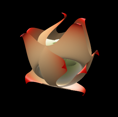
The applied colormap is shown below:

import numpy as np
import matplotlib.pyplot as plt
import s3dlib.surface as s3d
import s3dlib.cmap_utilities as cmu

# 1. Define function to examine ....................................
def planarfunc(xyz) :
    x,y,z = xyz
    r = np.sqrt( x**2 + y**2)
    Z = np.sin( 6.0*r )/2
    return x,y,Z

x_plane = lambda c : [ c[1],c[2],c[0] ]
y_plane = lambda c : [ c[2],c[0],c[1] ]
rad_dir = lambda c : s3d.SphericalSurface.coor_convert(c)[0]

# 2. Setup and map surface .........................................
rez = 6
cmap1 = cmu.hsv_cmap_gradient( 'darkgreen','cornsilk' )
cmap2 = cmu.hsv_cmap_gradient( 'cornsilk','red' )
cmap = cmu.stitch_cmap(cmap1,cmap2,name='grn_red')

wave_z = s3d.PlanarSurface(rez,'oct1').map_geom_from_op( planarfunc )
wave_x = s3d.PlanarSurface(rez,'oct1').map_geom_from_op( planarfunc )
wave_x.map_geom_from_op(x_plane)
wave_y = s3d.PlanarSurface(rez,'oct1').map_geom_from_op( planarfunc )
wave_y.map_geom_from_op(y_plane)

surface = wave_x + wave_y + wave_z
surface.map_cmap_from_op(rad_dir,cmap)

# 3. Construct figure, add surface, and plot ......................

fig = plt.figure(figsize=(4,4),facecolor='k')
ax = plt.axes(projection='3d', aspect='equal',facecolor='k')
ax.set_axis_off()
ax.view_init(-30,20)
s3d.auto_scale(ax,surface,rscale=0.7)
ax.add_collection3d(surface.shade(0.2,ax=ax).hilite())

fig.tight_layout(pad=0)
plt.show()