Spirals Surface

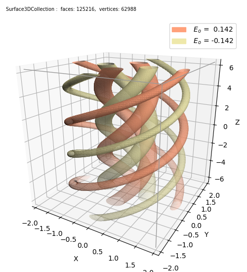
Given a scalar E, as a function of x,y, and z :

E_o = E(x,y,z)

Then the implicit surface, f, at a constant value of E_o is

f(x,y,z) = E(x,y,z) - E_o

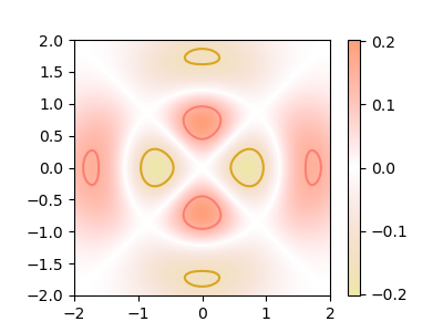
The above figure is an example of two surfaces, evaluated at two constant values. The functional form taken from Laser Resonators… . The values were selected by examinining the contours of the function at a constant value of z=0, as shown below:

import math
import numpy as np
from scipy import special as sp
import matplotlib.pyplot as plt
import matplotlib.patches as mpatches
import s3dlib.surface as s3d
import s3dlib.cmap_utilities as cmu

# 1. Define function to examine .....................................
def Exyz(xyz):
    p,l,isCos = 1,2,True
    r, theta, z = s3d.CylindricalSurface.coor_convert(xyz)
    sr2 = math.sqrt(2)
    Em = math.factorial(p)/math.factorial(p+l) # M(-n,a+1,x)
    L = sp.genlaguerre(p,l)
    E = Em*( ((sr2*r)**l) * L(2*r**2) * np.exp(-(r**2)) )
    if isCos:  E = E* (np.cos(l*theta-z))
    else:      E = E* (np.sin(l*theta-z))
    return E

# ................................
scol = ['lightsalmon', 'palegoldenrod']
dmn = [  [-2,2], [-2,2], [-2*np.pi,2*np.pi] ]
rez,Eo = 10, 0.142
Evals = [-Eo, Eo]

# 3D-plot ==========================================================

# 2. Setup and map surface .........................................

surface = s3d.Surface3DCollection.implsurf( Exyz, rez, dmn, *Evals, color=scol).evert()

# 3. Construct figure, add surface, and plot ......................
fig = plt.figure(figsize=(5,5.5))
fig.text(0.025,0.97,str(surface), ha='left', va='top', fontsize='x-small')
fig.text(0.5,.85,surface.name,ha='center',fontsize='x-large')
ax = plt.axes(projection='3d', aspect='equal', focal_length=0.25)
ax.view_init(20,-60)
s3d.auto_scale(ax,surface)
ax.set(xlabel='X',ylabel='Y',zlabel='Z')
E0_patch = mpatches.Patch(label=r'$\ E_o$ = '+str(Evals[0]), color=scol[0] )
E1_patch = mpatches.Patch(label=r'$\ E_o$ = '+str(Evals[1]), color=scol[1] )
ax.legend(handles=[E0_patch,E1_patch])
ax.add_collection3d( surface.shade(ax=ax).fade())
s3d.add_boxCorner(ax,dmn)

fig.tight_layout()

# XY-plot ==========================================================

def E_func(x,y) :
    z = np.zeros_like(x)
    xyz = np.array([x,y,z])
    return Exyz(xyz) 

N,colors = 100, ['salmon', 'goldenrod' ] 
    
# 2. Setup and map plane ...........................................

pg_wht = cmu.hsv_cmap_gradient(scol[0],'white')
wht_ls = cmu.hsv_cmap_gradient('white',scol[1])
pg_ls = cmu.stitch_cmap(pg_wht,wht_ls)

x = np.linspace(*dmn[0],N)
y = np.linspace(*dmn[1],N)
X,Y = np.meshgrid(x, y)
Z = E_func(X,Y)

# 3. Construct figure, add surface, and plot .......................

fig = plt.figure(figsize=(4,4))
ax = plt.axes( aspect='equal')
ax.set(xlabel='X',ylabel='Y', title='E(x,y,0)')

pos=ax.imshow(Z, cmap=pg_ls, extent=[*dmn[0],*dmn[1]])
CS = ax.contour(X, Y, Z, levels=Evals, colors=colors)
fig.colorbar(pos, ax=ax,  shrink=0.67)
fig.tight_layout()

# ==================================================================
plt.show()