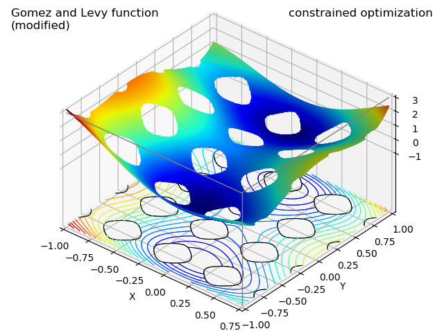
Clipping Surface and Contours

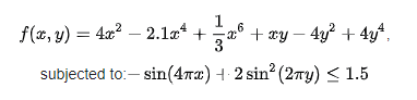
The function is given on the Wikipedia page Test functions for constrained optimization.

The function and constraint are given by:

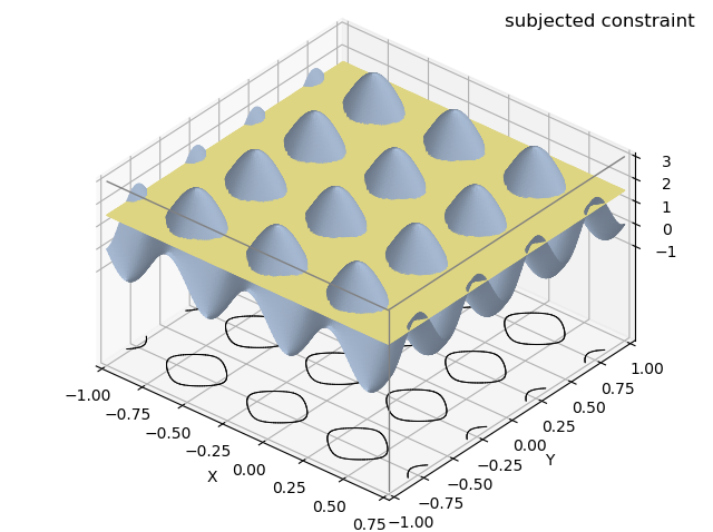
This example is a surface which is clipped using a functional operation, which itself is a function of a surface. The above ‘constrained optimization’ surface is clipped at the boundary intersection of a plane and ‘constraint’ surface. The ‘subjected constraint’ is visualized in the plot below.

The constrained optimization surface script is given below.

import numpy as np
import matplotlib.pyplot as plt
import s3dlib.surface as s3d

#.. Contours Projection and using a clipping function.

# 1. Define function to examine ....................................

def optimization(xyz) :
    x,y,z = xyz
    Z = 4*x**2 - 2.1*x**4 + x**6/3 + x*y - 4*y**2 + 4*y**4
    return x,y,Z

def constraint(xyz) :
    x,y,z = xyz
    Z = 2*(np.sin(2*np.pi*y))**2 - np.sin(4*np.pi*x)
    return x,y,Z

def criterion(xyz) :  return np.less_equal( constraint(xyz)[2] , 1.5)

# 2. Setup and map surface .........................................
rez=7

surface = s3d.PlanarSurface(rez,name='constrained optimization').domain( (-1,0.75) )
surface.map_geom_from_op(optimization)
surface.map_cmap_from_op( lambda xyz : xyz[2], 'jet')
contours = surface.contourLineSet(20)       #    | REQUIRED: Order Of Operation.
surface.clip(criterion)              # note-->   | Clip surface 'after' contours
contours.clip(criterion)             #           | are created, 'then' clip contours, 
contours.map_to_plane(-5)            #           | followed by projection.
contours.set_linewidth(0.75)

# ..... following is to form the black edges on the clipped contours...
c_surface = s3d.PlanarSurface(rez).domain( (-1,0.75) )  #.. note: not rendered
c_surface.map_geom_from_op(constraint)
c_contours = c_surface.contourLines(1.5, color='k')
c_contours.map_to_plane(-5)
c_contours.set_linewidth(0.75)

# ..... front grid ....................................................
vbox = [ [-1,-1,3],[0.75,-1,3],[0.75,1.0,3],[0.75,-1,-5] ]
ibox = [ [0,1,2],[1,3]]
box= s3d.ColorLine3DCollection(vbox,ibox,color='grey',linewidth=1)

# 3. Construct figure, add surface plot ............................

fig = plt.figure()
fig.text(0.975,0.975,surface.name, ha='right', va='top', fontsize='large')
sID = 'Gomez and Levy function\n(modified)'
fig.text(0.025,0.975,sID, ha='left', va='top', fontsize='large')
ax = plt.axes(projection='3d', proj_type='ortho')
ax.set(xlim=(-1,0.75), ylim=(-1,1), zlim=(-5,3) )
ax.view_init(38,-50)
ax.set_xlabel('X')
ax.set_ylabel('Y')
ax.set_xticks( (-1,-.75,-.50,-.25,0.0,0.25,0.5,0.75) )
ax.set_zticks( (-1,-.75,-.50,-.25,0.0,0.25,0.5,0.75,-1.0) )
ax.set_zticks( (-1,0,1,2,3) )

ax.add_collection3d(surface.shade(.5))
ax.add_collection3d(c_contours)
ax.add_collection3d(contours)
ax.add_collection3d(box)

fig.tight_layout()
plt.show()

The addition script for visualizing the constraint criterion is given below.

surface = s3d.PlanarSurface(rez, color='lightsteelblue' ).domain( (-1,0.75) )
surface.map_geom_from_op(constraint)
plane = s3d.PlanarSurface(rez, color='khaki').domain( (-1,0.75) )
plane.map_geom_from_op(lambda A : [ A[0], A[1], np.full(A.shape[1],1.5) ])
c_contours = surface.contourLines(1.5, color='k')
c_contours.map_to_plane(-5)
c_contours.set_linewidth(0.75)

surface = surface + plane
surface.name = 'subjected constraint'

vbox = [ [-1,-1,3],[0.75,-1,3],[0.75,1.0,3],[0.75,-1,-5] ]
ibox = [ [0,1,2],[1,3]]
box= s3d.ColorLine3DCollection(vbox,ibox,color='grey',linewidth=1)

fig = plt.figure()
fig.text(0.975,0.975,surface.name, ha='right', va='top', 
    fontsize='large', multialignment='right')
ax = plt.axes(projection='3d', proj_type='ortho')
ax.set(xlim=(-1,0.75), ylim=(-1,1), zlim=(-5,3) )
ax.view_init(38,-50)
ax.set_xlabel('X')
ax.set_ylabel('Y')
ax.set_xticks( (-1,-.75,-.50,-.25,0.0,0.25,0.5,0.75) )
ax.set_zticks( (-1,-.75,-.50,-.25,0.0,0.25,0.5,0.75,-1.0) )
ax.set_zticks( (-1,0,1,2,3) )

ax.add_collection3d(surface.shade(.5))
ax.add_collection3d(c_contours)
ax.add_collection3d(box)

fig.tight_layout()
plt.show()