Planar and Radial Contours

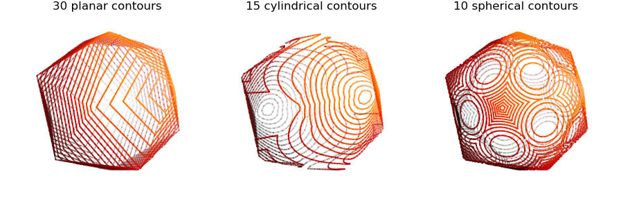
A custom colormap, leftGist, was constructed from the first 85% of the Matplotlib colormap gist_heat using the color map utilities function section_cmap.

This cmap was then used to ‘simulate’ a shading on the line contours using the line method map_cmap_from_op. This is similar to effect for normal shading on a sphere. However, there are no face normals to perform this surface operation for line segments.

The fade method was applied to create a sense of depth for the lines relative to the view orientation.

import numpy as np
from matplotlib import cm
from matplotlib import pyplot as plt
import s3dlib.surface as s3d
import s3dlib.cmap_utilities as cmu

#.. comparison of planar to spherical contours.

# 1. Define function to examine .....................................

def from_direction(xyz) :  return np.dot(xyz.T,[1,0,1])
cmu.section_cmap('gist_heat',0.0,.85,'leftGist')

# 2. Setup and map lines ............................................

surface = s3d.SphericalSurface.platonic(4)
lines = [None]*3
lines[0] = surface.contourLineSet(30,direction=[1,-.2,.5],coor=0,name='30 planar contours')
lines[1] = surface.contourLineSet(15,direction=[1,-.2,.5],coor=1,name='15 cylindrical contours')
lines[2] = surface.contourLineSet(10,                            name='10 spherical contours')

# 3. Construct figure, add surface, and plot ........................

minmax=(-0.65,0.65)
fig = plt.figure(figsize=(9,3))

for i in range(len(lines)) :
    ax = fig.add_subplot(1,3,1+i, projection='3d', aspect='equal')
    ax.set(xlim=minmax, ylim=minmax, zlim=minmax )
    ax.set_title(lines[i].name,  fontsize='large')
    ax.set_axis_off()
    lines[i].map_cmap_from_op(from_direction,'leftGist').fade()

    ax.add_collection3d(lines[i])

fig.tight_layout()
plt.show()