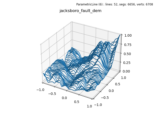
Datagrid Slices

import numpy as np
import matplotlib.pyplot as plt
from matplotlib.ticker import LinearLocator
from mpl_toolkits.mplot3d import axes3d
import s3dlib.surface as s3d

#.. Datagrid surface and xySlice line set plot

# 1. Define function to examine .....................................
z=np.load('data/jacksboro_fault_dem.npz')['elevation']
datagrid = np.flip( z[5:50, 5:50], 0 )

# 2. Setup and map surfaces .........................................
rez=6

line = s3d.ParametricLine(rez, cmap='gist_earth', name='jacksboro_fault_dem')
line.map_xySlice_from_datagrid(datagrid, yset=50,xset=2).shade(0.7)

# 3. Construct figure, add surface, plot ............................
fig = plt.figure()
ax = plt.axes(projection='3d')

fig.text(0.975,0.975,str(line), ha='right', va='top', fontsize='smaller')
fig.text(0.025,0.025,line.cname, ha='left', va='bottom', fontsize='smaller')
ax.set_title( line.name )

ax.set(xlim=(-1,1), ylim=(-1,1), zlim=(0,1) )
ax.xaxis.set_major_locator(LinearLocator(5))
ax.yaxis.set_major_locator(LinearLocator(5))
ax.zaxis.set_major_locator(LinearLocator(5))

ax.add_collection3d(line)

plt.show()

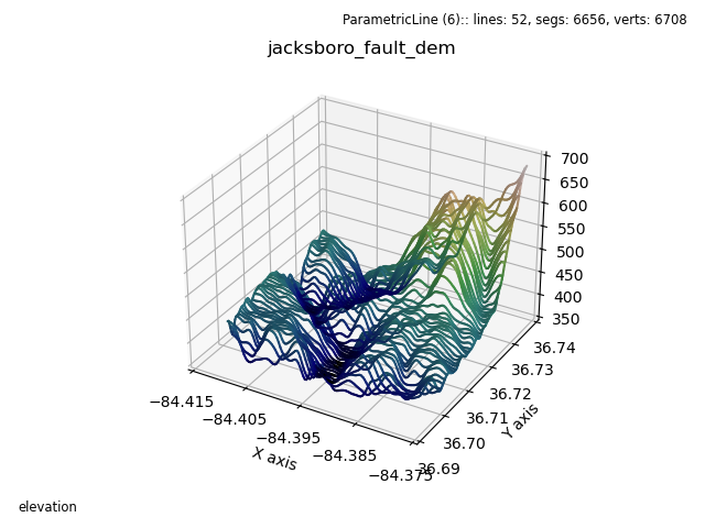
Vertical Colorization

The referenced matplotlib example uses a cmap applied to the vertical location of the surface. This can also be easily constructed similar to Vertical Colorization of the surface with the resulting plot shown below.

import numpy as np
import matplotlib.pyplot as plt
from matplotlib.ticker import LinearLocator
from mpl_toolkits.mplot3d import axes3d
import s3dlib.surface as s3d

#.. Datagrid xySlice line set plot

# 1. Define function to examine .....................................

with np.load('data/jacksboro_fault_dem.npz') as dem :
    z = dem['elevation']
    nrows, ncols = z.shape
    x = np.linspace(dem['xmin'], dem['xmax'], ncols)
    y = np.linspace(dem['ymin'], dem['ymax'], nrows)
    x, y = np.meshgrid(x, y)

region = np.s_[5:50, 5:50]
x, y, z = x[region], y[region], z[region]

datagrid = np.flip(z,0)

# 2. Setup and map surfaces .........................................
rez=6

line = s3d.ParametricLine(rez, cmap='gist_earth', name='jacksboro_fault_dem')
line.map_xySlice_from_datagrid(datagrid, yset=50,xset=2)
line.map_cmap_from_op(lambda xyz:  xyz[2], cname='elevation').shade(0.7)
line.scale_dataframe(x,y,datagrid)

# 3. Construct figure, add surface, plot ............................
fig = plt.figure()
ax = plt.axes(projection='3d')

fig.text(0.975,0.975,str(line), ha='right', va='top', fontsize='smaller')
fig.text(0.025,0.025,line.cname, ha='left', va='bottom', fontsize='smaller')
ax.set_title( line.name )

ax.set(xlim=(-84.415,-84.375), ylim=(36.690,36.740), zlim=(350,700) )

ax.xaxis.set_major_locator(LinearLocator(5))
ax.yaxis.set_major_locator(LinearLocator(6))
ax.zaxis.set_major_locator(LinearLocator(8))
ax.set_xlabel('X axis')
ax.set_ylabel('Y axis')

ax.add_collection3d(line)

plt.show()