Scalar Function Colormapping on a 3D Surface

This example is based on the Matplotlib function used in the Hillshading example.

For this case, the function domain and range are clear in a 3D visualization and as a result, a colorbar is not shown. To enhance the shading, the map_cmap_from_normals and shade methods are applied to the surface.

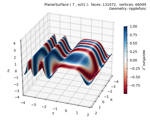
The following applies this function’s scalar z-value, represented using a colormap, on an alternative geometry. For this latter case, a colorbar is needed to interpret the scalar value.

import numpy as np
from matplotlib import pyplot as plt
import s3dlib.surface as s3d

#.. Cmapped Normals, Shading and Highlighting

# 1. Define function to examine .....................................
rez=7

def wavefunc(xyz) :
    x,y,z = xyz
    Z = np.cos( x**2 + y**2 )
    return x,y,Z

def ripplefunc(xyz) :
    x,y,z = xyz
    Z = np.cos( y**2 )
    return x,y,Z

def wavefunc_z(xyz) : return wavefunc(xyz)[2]

# Figure 1 - wavefunc geometry ======================================

wave = s3d.PlanarSurface(rez, basetype='oct1').domain([-4,2],[-4,2])
wave.map_geom_from_op( wavefunc )
wave.map_cmap_from_normals('copper').shade().hilite(focus=2)

# 3. Construct figure, add surface, plot ............................

fig = plt.figure(figsize=plt.figaspect(0.9))
info = str(wave) + '\nGeometry: ' + wave.name
fig.text(0.975,0.975,info, ha='right', va='top', multialignment='right')
ax = plt.axes(projection='3d')
ax.set( xlim=(-4,2), ylim=(-4,2), zlim=(-4,4),
    xlabel='X', ylabel="Y", zlabel="Z"  )
ax.view_init( azim=20 )

ax.add_collection3d(wave)

fig.tight_layout()

# Figure 2 - ripplefunc geometry, wavefunc color ======================

ripple = s3d.PlanarSurface(rez, basetype='oct1', cmap='RdBu').domain([-4,2],[-4,2])
ripple.map_cmap_from_op( wavefunc_z )
ripple.map_geom_from_op( ripplefunc ).shade(direction=[0,0,1])
ripple.hilite(1,direction=[.3,.3,1],focus=2)

# 3. Construct figure, add surface, plot ............................

fig = plt.figure(figsize=plt.figaspect(0.8))
info = str(ripple) + '\nGeometry: ' + ripple.name
fig.text(0.975,0.975,info, ha='right', va='top', multialignment='right')
ax = plt.axes(projection='3d')
ax.set( xlim=(-4,2), ylim=(-4,2), zlim=(-4,4),
    xlabel='X', ylabel="Y", zlabel="Z"  )
ax.view_init( azim=20 )
cbar = plt.colorbar(ripple.cBar_ScalarMappable, ax=ax,  shrink=0.6, pad=-0.05 )
cbar.set_label(ripple.cname, rotation=270, labelpad = 15)

ax.add_collection3d(ripple)

fig.tight_layout()

# =====================================================================

plt.show()