Vertical Contour Set

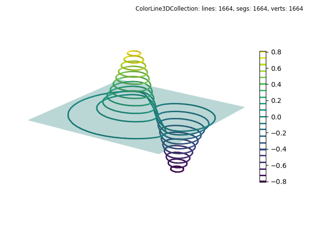
Contours were created using the surface geometry from the Hello World Example example. A striped colormap was generated using the stcBar_ScalarMappable line method shown in the highlighted line.

import numpy as np
import matplotlib.pyplot as plt
import s3dlib.surface as s3d
from matplotlib import colormaps

### see demo_A

# 1. Define function to examine .....................................

def geo_map(xyz) :
    x,y,z = xyz
    X,Y = 3*x, 3*y
    Z1 = np.exp(-X**2 - Y**2)
    Z2 = np.exp(-(X - 1)**2 - (Y - 1)**2)
    Z = Z1-Z2
    return x,y,Z

# 2. Setup and map surfaces .........................................
rez = 5
pc = colormaps['viridis'](0.5)

plane = s3d.PlanarSurface(color=pc).set_surface_alpha(.3)

surface = s3d.PlanarSurface(rez)
surface.map_geom_from_op( geo_map )

line = surface.contourLineSet(21)
line.map_cmap_from_op(lambda xyz: xyz[2])
line.set_linewidth(2)

# 3. Construct figure, add surface, plot ............................

fig = plt.figure(figsize=plt.figaspect(0.75))
fig.text(0.975,0.975,str(line), ha='right', va='top', fontsize='smaller', multialignment='right')
ax = plt.axes(projection='3d', aspect='equal')
minmax = ( -0.8,0.8 )
ax.set(xlim=minmax, ylim=minmax, zlim=minmax )
plt.colorbar(line.stcBar_ScalarMappable(21,'w'), ax=ax,  shrink=0.6 )
ax.set_axis_off()
ax.view_init(20,-55)

ax.add_collection3d(plane.shade())
ax.add_collection3d(line.shade(.7))

fig.tight_layout()
plt.show()

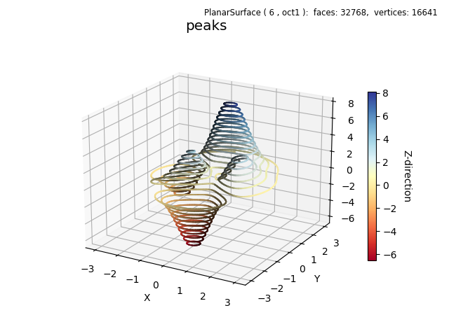
Instead of coloring the contours directly, contours will take the color of the surface from which it is constructed. Using the Peaks example script, instead of adding the surface to the axis, contours are added using:

ax.add_collection3d(surface.shade().contourLineSet(25))

to produce the following figure: