Unstructured Spherical and Cylindrical Coordinates

Using an unstructured dataset in spherical coordinates is similar to using a planar coordinated system shown in Unstructured coordinates example.

Also, surfaces from datasets which include additional vertex values are shown in the Unstructured Spherical Dataset and Unstructured Cylindrical Dataset examples.

import numpy as np
import matplotlib.pyplot as plt
from matplotlib import colormaps,colors
import s3dlib.surface as s3d

#.. Unstructured spherical coordinates

sixColors = colormaps['Blues'](np.linspace(0, 1, 6))
sixColor_cmap = colors.ListedColormap(sixColors)

# make data:  <--- copy from matplotlib examples
np.random.seed(1)
x = np.random.uniform(-3, 3, 256)
y = np.random.uniform(-3, 3, 256)
z = (1 - x/2 + x**5 + y**3) * np.exp(-x**2 - y**2)

# transform to a spherical dataset, (r,t,p)
t = (x/3 +1)*np.pi
p = (y/3 +1)*np.pi/2
r = z + 2   # <-- shift the radius
rtp = np.array([r,t,p])
xyz = s3d.SphericalSurface.coor_convert(rtp,True)  # <-- for scatter plot

# 2. Setup and map surface .........................................

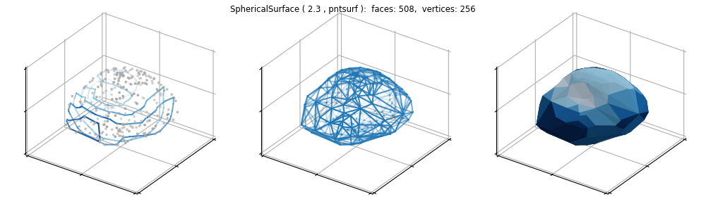
surface = s3d.SphericalSurface.pntsurf(rtp.T)
edges = surface.edges
surface.map_cmap_from_op( cmap='Blues') # <-- to set contour colors, next
contours = surface.contourLineSet(5) # default: spherical contours
surface.map_cmap_from_op( cmap=sixColor_cmap)

# 3. Construct figure, add surface, and plot ......................

fig = plt.figure(figsize=(10,3))
fig.text(0.5,0.975,str(surface), ha='center', va='top', fontsize='smaller')
minmax,ticks = (-3,3), [-3,0,3]
for i in range(3) :
    ax = fig.add_subplot(131+i, projection='3d')
    ax.set(xticks=ticks,yticks=ticks,zticks=ticks,
            xlim=minmax, ylim=minmax, zlim=minmax ) 
    ax.tick_params(labelcolor='w')
    ax.set_proj_type('ortho')
    ax.xaxis.set_pane_color([1,1,1])
    ax.yaxis.set_pane_color([1,1,1])
    ax.zaxis.set_pane_color([1,1,1])
    ax.view_init(azim=-145)
    if i==0 : ax.scatter(*xyz, s=3, c='darkgrey')
    ax.add_collection3d(contours.fade(0.3,ax=ax) \
    if i==0 else edges.fade(0.1,ax=ax) if i==1 else surface.shade(.4,ax=ax))

fig.tight_layout(pad=0)

plt.show()

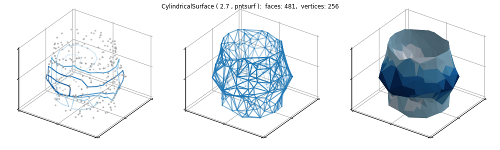
Using a cylindrical dataset results in the following.

The only change to the script to produce the 3D figure in cylindrical coordinates is the following:

# transform to a cylindrical dataset, (r,t,z)
t = (x/3 +1)*np.pi
Z = y
r = z + 2   # <-- shift the radius
rtz = np.array([r,t,Z])
xyz = s3d.CylindricalSurface.coor_convert(rtz,True)  # <-- for scatter plot

# 2. Setup and map surface .........................................

surface = s3d.CylindricalSurface.pntsurf(rtz.T)
edges = surface.edges
surface.map_cmap_from_op( cmap='Blues') # <-- to set contour colors, next
contours = surface.contourLineSet(5) # default: cylincrical contours
surface.map_cmap_from_op( cmap=sixColor_cmap)

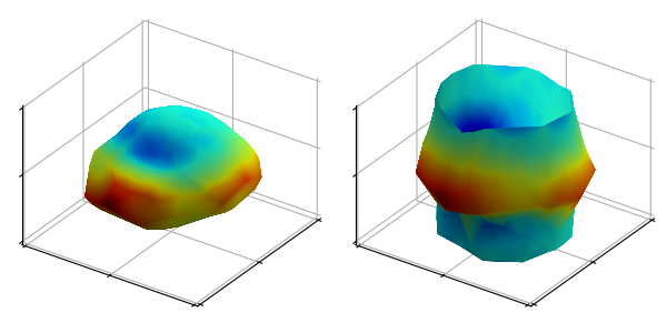
These visualization are enhanced using a varying hue colormap instead of uniform hue, as shown below. The number of contours was increased from 5 to 10 to further enhance the interpretation.

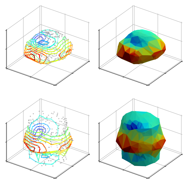
Similar to the Unstructured coordinates, Smoothed Surface example, geometric and color smoothing is made using:

    surface.triangulate(4)
    surface.map_cmap_from_op(cmap='jet')
    surface.shade(.3,flat=False)

to produce the result: