Selecting a Base

As seen in the Summary Table, a variety of native coordinates and surface base types are available. Why so many? The variety is to generalize possible surfaces which may be visualized.

Selecting the optimal base surface may not be obvious. Intuitively, if the surface ‘looks’ like a squashed sphere, a SphericalSurface object would probably be the best choice. However, for complex functional relationships, optimal selection will depend on:

1. The native coordinate system

   • functional description
   • functional domain
   • surface symmetry
   • degree of local surface curvature

2. Optimal uniformity in

   • vertex distribution
   • triangular face areas and shapes

3. Shape and distribution of surface faces considering

   • surface clipping
   • application of color operations and mapping

Most surface subclass bases have been formulated so that the surface faces are of uniform shape and size. As a result, using a subclass object that transforms to preserve the overall ‘shape’ is often the best starting object. For example, a surface with axial symmetry about the z-axis is best represented using a surface object with an axial coordinate, rather than a PlanarSurface object. Also, the functional description is easier to apply and to interpret if it is described in the native coordinates.

In addition, numerous geometries were developed to accommodate geometric mapping using:

1. Functions with a singularity at the origin. For polar and spherical basetypes, using the minrad argument may be used to exclude vertex coordinates a limited distance from the origin.
2. Functions which are not cyclic in the angular domain, f(0) ≠ f(2π) or which have an extended domain beyond 2π. The ‘split’ basetype geometries provide unconnected faces at the azimuthal angle θ at 0 and 2π.
3. Functions describing non-orientable surfaces. Split basetype geometries are also useful for these cases.
4. Functions exhibiting various forms of symmetry. Circumferential basetypes are convenient to explicitly set the distribution of polyhedron faces based on functional symmetries. For example, see Hello World Example 2.

Bottom line: first, select a convenient coordinate system applicable to the functional descriptions. Then guess which basetype and rez. These are easy to change into one line in the object constructor. Finally, examine the effect and change these values to improve the visualization.

Native Coordinates

Each of the surface classes have a native coordinate system which is convenient for further geometric or color mapping. The choice of the base is dependent on both these two. In the following figure, a ‘simple’ example shows similar surfaces but can be developed for different purposes.

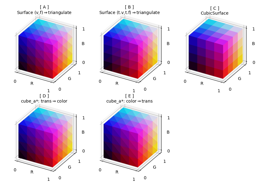
In the above figure, the native coordinate for the top row surfaces is xyz whereas the bottom row uses spherical rtp coordinates. For these examples:

1. The base class is instantiated with explicitly defined vertex coordinates and face indices. Any further geometric transform function will use xyz coordinate arguments and return value. The Base Class Geometric Mapping example uses this construction method and, as such, the transform function uses these coordinates.
2. As with the previous example, the base class is used to create the surface object. However, for this case, vertex and indices are taken from a previously constructed surface. This technique may be used for any surface type which doesn’t necessarily have xyz coordinates. The Double Planetoid example uses this construction method.
3. For simple ‘cubic-type’ geometries, the CubicSurface class is the obvious choice. However, further geometric mapping is limited to linear transforms since the faces are rectangular. For non-linear mapping, the surface should be triangulated prior to mapping. The 3D Box Surface Plot example uses this construction method.
4. The SphericalSurface class is used to initially construct the surface for the cube platonic solid. The cube-shaped surface is transformed to the position where rgb corresponds to xyz. Then the xyz-coordinates are directly color mapped. The Color Space HSV example uses cylindrical coordinates to map to colors directly from hsv color space.
5. As with the previous example, the SphericalSurface class is used to construct the surface. In this case, the color mapping function uses the native rtp coordinates, then moved to the [0,1] domain. This is similar to the Functional RGB Color Mapping example.

The base class chosen can reduce the transformational code development through the use of convenient native coordinates used for mapping operations. For example, Lab Planes plots utilize five different base classes, dependent on the intended mapping to produce the final surface geometry.

Note

The triangulate method subdivides each triangle into smaller triangles within the triangle plane. This method, by itself, will have no visual effect on the geometry. However, since each triangle in Matplotlib rendering will have a uniform color, variations in color mapping can be visualized within the original subdivided face. In addition, further geometric mapping of the surface can be made which will change the planar geometry of the original face.

The figures were constructed from the script:

import numpy as np
import matplotlib.pyplot as plt
import s3dlib.surface as s3d

#.. Comparison of RGB cube construction.

# 1. Define functions to examine ========================================

v = [   [  0, 0, 0 ],  [  0, 1, 0 ],  [ 1 , 1, 0 ],  [  1, 0, 0 ],
        [  0, 0, 1 ],  [  0, 1, 1 ],  [ 1 , 1, 1 ],  [  1, 0, 1 ]  ]
f = [ [0,1,2,3], [3,2,6,7], [2,1,5,6], [1,0,4,5], [0,3,7,4], [4,7,6,5] ]

def toRGB(rtp) :
    xyz = s3d.SphericalSurface.coor_convert(rtp,True)
    return (np.ones_like(xyz)+xyz)/2

# 2. Setup and map surfaces =============================================
rez,cube = 2, [None]*5

# Surface3DCollection Base Class 1 ....................................
title = '[ A ]\nSurface (v,f)'+ r'$\Rightarrow$triangulate'
cube[0] = s3d.Surface3DCollection(v, f, name=title).triangulate(rez)
cube[0].map_color_from_op(lambda xyz : xyz)

# Surface3DCollection Base Class 2 ....................................
title = '[ B ]\nSurface (t.v,t.f)'+ r'$\Rightarrow$triangulate'
t = s3d.SphericalSurface.platonic(0,'cube_a',name=title).domain(.5)
t.transform(translate=[0.5,0.5,0.5])
v, f = t.vertexCoor, t.fvIndices
cube[1] = s3d.Surface3DCollection(v, f, name=title).triangulate(rez)
cube[1].map_color_from_op(lambda xyz : xyz)

# CubicSurface Class ..................................................
title = '[ C ]\nCubicSurface'
cube[2] = s3d.CubicSurface(rez, name=title)
cube[2].domain( [0,1],[0,1],[0,1] )
cube[2].map_color_from_op(lambda xyz : xyz)

# SphericalSurface Class : Transform => Color .........................
title = '[ D ]\ncube_a*: '+ r'trans$\Rightarrow$color'
cube[3] = s3d.SphericalSurface.platonic(rez,'cube_a',name=title).domain(.5)
cube[3].transform(translate=[0.5,0.5,0.5])
cube[3].map_color_from_op(lambda rtp : s3d.SphericalSurface.coor_convert(rtp,True))

# SphericalSurface Class : Color => Transform .........................
title = '[ E ]\ncube_a*: '+ r'color$\Rightarrow$trans'
cube[4] = s3d.SphericalSurface.platonic(rez,'cube_a',name=title)
cube[4].map_color_from_op(toRGB)
cube[4].transform(translate=[1,1,1]).transform(scale=0.5)  

# 3. Construct figure, add surfaces, and plot ===========================

rgb_minmax, rgb_ticks = (-0.05,1.05) , [0,1]
fig = plt.figure(figsize=(8.5,6))

for i,rgb_cube in enumerate(cube) :
    ax = fig.add_subplot(231+i, projection='3d')
    ax.set_aspect('equal')
    ax.set(xlim=rgb_minmax, ylim=rgb_minmax, zlim=rgb_minmax)
    ax.set_xticks(rgb_ticks)
    ax.set_yticks(rgb_ticks)
    ax.set_zticks(rgb_ticks)
    ax.set_xlabel('R', labelpad=-10)
    ax.set_ylabel('G', labelpad=-10)
    ax.set_zlabel('B', labelpad=-10)
    ax.set_proj_type('ortho')
    ax.set_title( rgb_cube.name, fontsize='medium' )

    ax.add_collection3d(rgb_cube.shade(.5))

fig.tight_layout(pad=2)
plt.show()

Face and Vertex Distribution

Instead of interpreting the subclass objects as surface geometries, it can be advantageous to consider the objects in terms of a graph of interconnected vertices and edges. The set of vertices are defined within the point domain of two independent variables. For the subclass objects:

Graph (Class)	Independent Variable
PlanarSurface	( x,y )
PolarSurface	( r, θ )
CylindricalSurface	( θ, z )
SphericalSurface	( θ , φ )

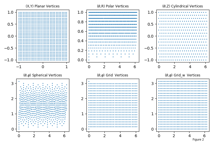
With appropriate mapping, each of these ‘graphs’ can be transformed into a similar surface. Consider the simple example of a sphere. A usual method of developing a grid to construct the surface is to uniformly subdivide the angular and azimuthal coordinates. Alternatively using S3Dlib, the six different ‘graphs’ can be used to visualize the sphere, as shown below. The number in each plot title represents the number of vertices.

Using a SphericalSurface object, vertices are distributed so that the triangular faces are relatively uniform by design, without a concentration of elongated faces near the poles. For the other three objects, faces are not uniform and face anomalies may also occur at the poles since multiple vertices are formed at these two locations.

Vertex Coordinates

For complex functional mapping involving parametric equations, a uniform vertex distribution may be preferable. The vertex distribution of these six surfaces is

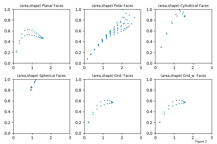
Face Size and Shape

The face shape and size distributions will depend on the base surfaces and subsequent geometric mapping. These distributions are compared for the surface sizes in the following figures. The areas are normalized to the average face areas. The shapes are normalized so that equilateral triangles and squares shapes are one.

The following is a comparison among the general spherical base shapes at different rez values, and rectangular grid-based shapes at different subdivision sizes. This provides a comparison for initial geometries, independent of subsequent geometric mapping.

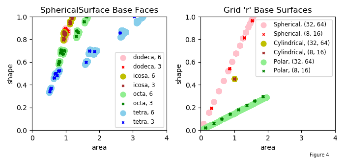
Several observations:

1. the rez has a minimal influence on the area-shape distribution of the surface.
2. uniform faces are located near the (1,1) coordinate in this plot.
3. increases in rez will most affect the geometric uniformity of the visualization for surfaces with faces at the right of the plot. (large areas)
4. increases in rez will most affect the color uniformity of the visualization for surfaces with faces at the lower part plot. (distorted shapes)
5. for rectangular faced cylindrical grids, the relative areas are always one and the face shape only depends on the ratio of the subdivisions. For polar and spherical grid base types, the linear slope on these plots depends on the subdivision’s ratio.

The above four figures were constructed from the script:

import numpy as np
from matplotlib import pyplot as plt
import s3dlib.surface as s3d
import s3dlib.cmap_utilities as cmu

#.. sphere vs planar, polar, cylindrical, sphere and globe vertices

# 1. Define function to examine .....................................

def plane2sphere(xyz) :
    x,y,z = xyz
    T = -np.pi*(x+1)
    P = np.pi*(y+1)/2
    R = np.ones(len(z)).astype(float)
    XYZ = s3d.SphericalSurface.coor_convert([R,T,P],True)
    return XYZ

def disk2sphere(rtz) :
    r,t,z = rtz
    P = np.pi*r
    R = np.ones(len(z)).astype(float)
    XYZ = s3d.SphericalSurface.coor_convert([R,t,P],True)
    return XYZ

def cylinder2sphere(rtz) :
    r,t,z = rtz
    P = np.pi*(z+1)/2
    t = -t
    XYZ = s3d.SphericalSurface.coor_convert([r,t,P],True)
    return XYZ

# 2. Setup and map surfaces .........................................
rez = 3
cmap = cmu.rgb_cmap_gradient([0.25,0.15,0],[1,.9,.75])

plane = s3d.PlanarSurface(rez+1,basetype='oct1')
x,y,z = plane.vertices
plane.map_geom_from_op( plane2sphere )
plane.map_cmap_from_normals(cmap).shade()

disk = s3d.PolarSurface(rez+1,basetype='hex')
rp,tp,zp = s3d.PolarSurface.coor_convert(disk.vertices)
disk.map_geom_from_op( disk2sphere,True )
disk.map_cmap_from_normals(cmap).shade()

cylinder = s3d.CylindricalSurface(rez,basetype='tri')
rc,tc,zc = s3d.CylindricalSurface.coor_convert(cylinder.vertices)
cylinder.map_geom_from_op( cylinder2sphere,True )
cylinder.map_cmap_from_normals(cmap).shade()

sphere = s3d.SphericalSurface(rez,basetype='icosa')
rs,ts,ps = s3d.SphericalSurface.coor_convert(sphere.vertices)
sphere.map_cmap_from_normals(cmap).shade()

globe = s3d.SphericalSurface.grid(20,34)
rg,tg,pg = s3d.SphericalSurface.coor_convert(globe.vertices)
globe.map_cmap_from_normals(cmap).shade()

globes = s3d.SphericalSurface.grid(20,34, 'w',minrad=0.001)
rz,tz,pz = s3d.SphericalSurface.coor_convert(globes.vertices)
globes.map_cmap_from_normals(cmap).shade()

surfaces = [
    [ plane,    [x,y],    '(X,Y)',                'Planar' ],
    [ disk,     [tp,rp], r'($\theta$,R)',         'Polar' ],
    [ cylinder, [tc,zc], r'($\theta$,Z)',         'Cylindrical' ],
    [ sphere,   [ts,ps], r'($\theta$,$\varphi$)', 'Spherical' ],
    [ globe,    [tg,pg], r'($\theta$,$\varphi$)', 'Grid ' ] ,
    [ globes,   [tz,pz], r'($\theta$,$\varphi$)', 'Grid_w ' ] ]

# 3. Construct figure, add surface, plot ............................

# Figure 1 Spherical surface views .........................

fig = plt.figure(figsize=(6,4))
fig.text(0.9,0.01,'Figure 1', fontsize='x-small')
minmax = ( -0.7,0.7 )
for i in range(len(surfaces)) :
    surface = surfaces[i]
    ax = fig.add_subplot(231+i, projection='3d')
    ax.set_aspect('equal')
    ax.set(xlim=minmax, ylim=minmax, zlim=minmax )
    title = surface[3] + 'Surface, ' + str(len(surface[0].vertices[0]))
    ax.set_title( title, fontsize='medium' )
    ax.set_axis_off()
    ax.set_proj_type('ortho')
    ax.view_init(0)
    ax.add_collection3d(surface[0])

fig.tight_layout()

# Figure 2 - Vertex distribution plots .....................

fig = plt.figure(figsize=(7.5,5))
fig.text(0.9,0.01,'Figure 2', fontsize='x-small')
for i in range(len(surfaces)) :
    surface = surfaces[i]
    ax = fig.add_subplot(231+i)
    title = surface[2] +' '+ surface[3] +' Vertices'
    ax.set_title( title , fontsize='small' )
    x,y = surface[1]
    ax.scatter(x,y,s=1)

fig.tight_layout(pad=1)

# Figure 3 - Area distribution plots .....................

fig = plt.figure(figsize=(7.5,5))
fig.text(0.9,0.01,'Figure 3', fontsize='x-small')
for i in range(len(surfaces)) :
    surface = surfaces[i][0]
    ax = fig.add_subplot(231+i)
    title = '(area,shape) ' + surfaces[i][3] +' Faces'
    ax.set_title( title , fontsize='small' )
    a,s = surface.area_h2b
    ax.set(xlim=(0,3), ylim=(0,1))
    ax.scatter(a,s,s=1)

fig.tight_layout(pad=1)

# Figure 4 - Comparison of basetype and rez .....................

color = ['pink','r','y','brown','lightgreen','g','skyblue','blue']

baseTypes = [
    ['dodeca','icosa','octa','tetra'],
    ['Spherical','Cylindrical','Polar']
    ]
classes = [ s3d.SphericalSurface, s3d.CylindricalSurface, s3d.PolarSurface ]
title = ["SphericalSurface Base Faces", "Grid 'r' Base Surfaces"]

fig = plt.figure(figsize=(7,3.25))
fig.text(0.9,0.01,'Figure 4', fontsize='x-small')
for j in range(2) :
    bases = baseTypes[j]
    ax = fig.add_subplot(121+j)
    for i in range(2*len(bases)) :
        btype = bases[int(i/2)]
        size =  60 if i%2==0 else 10
        mark = 'o' if i%2==0 else 'x'
        if j == 0 :
            rez  =   6 if i%2==0 else 3
            label = btype +', '+ str(rez)
            surf = s3d.SphericalSurface(rez,btype)
        else :
            grez = 4 if i%2==0 else 1
            label = btype +', '+ str((grez*8,grez*16))
            surf = classes[int(i/2)].grid(grez*8,grez*16,'r')
        a,k = surf.area_h2b
        ax.scatter(a,k,s=size,marker=mark,c=color[i],label=label)
    ax.set_title(title[j])
    ax.set(xlim=(0,4), ylim=(0,1),xlabel='area', ylabel='shape')
    ax.legend(fontsize='small')
fig.tight_layout(pad=1)

# ..........................................................
plt.show()

In the above functions plane2sphere and cylinder2sphere, the T variable is set negative. This is to have a consistent outward normal to the faces using a right-hand rule definition.

Mapping ℝ³ → ℝ² → ℝ³

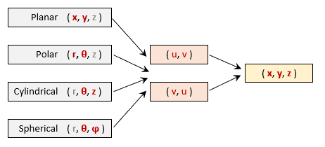
Parametric surfaces from graphs of functions of two variables, f(u,v), are directly constructed from the base surface geometries by mapping the two surface independent variables.

The triangular face shapes and sizes of the resulting mapped surface will depend on the vertex distribution of the initial base surface which is controlled by:

• surface coordinate system
• basetype or circumferential geometries
• split geometries and minrad parameter
• mapping domain

Often for complex geometries, the final spatial distribution of faces is not obvious beforehand. A major advantage of using S3Dlib is that surface geometries are set in one expression. Therefore, during code development, effects of geometry can be easily evaluated and alternatives can be made. In addition, each subclass has the coor_convert method to transform among planar, polar, cylindrical and spherical coordinates. The Complex Number Representation, Geometry and Colormap example shows visualizations for the same function using polar, planar and cylindrical coordinates.

This provides flexibility to evaluate the visualization for different grids. For example, the Klein Bottle, Spherical to XYZ example uses a SphericalSurface object. This parametric surface can be constructed from any of the surface objects, with the resulting visualization dependent on the distribution of the vertices.

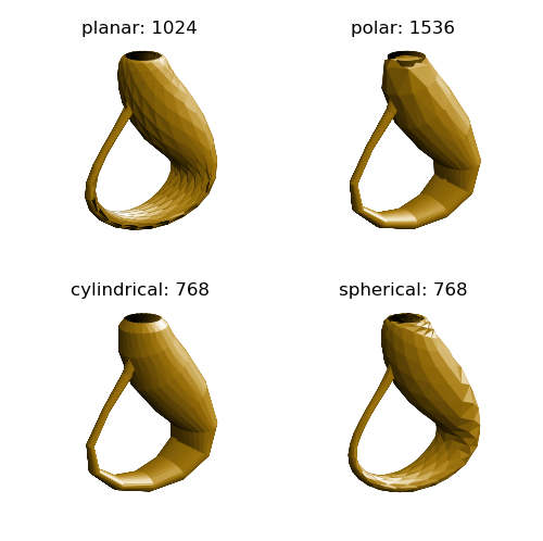
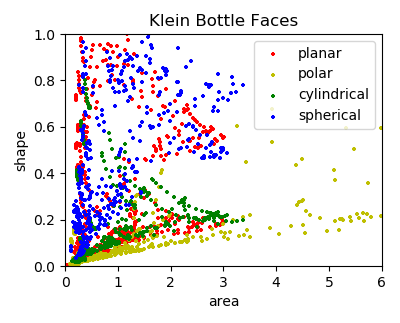
For each coordinate system geometry, a function defines the transform from the two base surface independent variables to the two parametric surface variables. From the area-shape plot, the planar and spherical bases would provide a ‘smoother’ surface with points more to the upper left. For the above plots, the highlighted code lines in the script below are the mapping functions.

import numpy as np
from matplotlib import pyplot as plt
import s3dlib.surface as s3d

#.. Klein Bottle using various base systems

# 1. Define function to examine ....................................

def planar_klein(xyz) :
    x,y,z = xyz
    v = -np.pi*(x+1)
    u = np.pi*(y+1)/2
    return klein_UV(u,v)

def polar_klein(rtz) :
    r,t,z = rtz
    u = np.pi*r
    v = t
    return klein_UV(u,v)

def cylin_klein(rtz) :
    r,t,z = rtz
    u = np.pi*(z+1)/2
    v = -t
    return klein_UV(u,v)

def sphere_klein(rtp) :
    r,t,p = rtp
    u = t/2
    v = -2*p
    return klein_UV(u,v)

# ================================

def klein_UV(u,v) :
    # domain :  0 < u < pi
    #           0 < v < 2*pi
    cU, sU = np.cos(u), np.sin(u)
    cV, sV = np.cos(v), np.sin(v)
    x = -(2/15)*cU* \
        (  ( 3 )*cV + \
           ( -30 + 90*np.power(cU,4) - 60*np.power(cU,6) + 5*cU*cV )*sU \
        )
    y = -(1/15)*sU* \
        (  ( 3 - 3*np.power(cU,2) -48*np.power(cU,4) +48*np.power(cU,6) )*cV + \
           (-60 + ( 5*cU - 5*np.power(cU,3) - 80*np.power(cU,5) + 80*np.power(cU,7) )*cV  )*sU \
        )
    z = (2/15)*( 3 + 5*cU*sU )*sV
    return x,y,z

# 2. Setup and map surface .........................................
rez,lw,color = 3, 1, 'darkgoldenrod'
bottles = [None]*4

klein = s3d.PlanarSurface(rez+1,color=color,lw=lw, name='planar' )
bottles[0] = klein.map_geom_from_op( planar_klein )

klein = s3d.PolarSurface( rez+1,color=color,lw=lw, name='polar' )
bottles[1] = klein.map_geom_from_op( polar_klein, returnxyz=True )

klein = s3d.CylindricalSurface(rez,color=color,lw=lw, name='cylindrical' )
bottles[2] = klein.map_geom_from_op( cylin_klein, returnxyz=True )

klein = s3d.SphericalSurface(rez,basetype='cube_c',color=color,lw=lw, name='spherical' )
bottles[3] = klein.map_geom_from_op( sphere_klein, returnxyz=True )

# 3. Construct figure, add surface plot ............................

# Figure 1 Klein bottle surface views .............................

fig = plt.figure(figsize=(5,5))
minmax = (-1.5,1.5)
vdir = s3d.rtv([-1,-1,-1],20,-125)
for i in range(4) :
    ax = fig.add_subplot(221+i, projection='3d')
    ax.set_aspect('equal')
    ax.set(xlim=minmax, ylim=minmax, zlim=minmax)
    ax.set_axis_off()
    ax.view_init(elev=20, azim=-125)
    bottle = bottles[i]
    bottle.transform(s3d.eulerRot(0,-90),translate=[0,0,2])
    bottle.shade( direction=vdir ).hilite(direction=vdir)
    ax.set_title(bottle.name+': '+ str(len(bottle.facecenters[0]) ) )
    ax.add_collection3d(bottle)
fig.tight_layout()

# Figure 2 Klein bottle area distribution plots ...................

color = ['r','y','g','blue']
fig = plt.figure(figsize=(4,3.25))
ax = plt.axes()
for i in range(len(bottles)) :
    bottle = bottles[i]
    label = bottle.name
    a,k = bottle.area_h2b
    ax.scatter(a,k,s=5,marker='+',c=color[i],label=label)
ax.set_title('Klein Bottle Faces')
ax.set(xlim=(0,6), ylim=(0,1),xlabel='area', ylabel='shape')
ax.legend()
fig.tight_layout(pad=1)

# ..................................................................
plt.show()

Note

For parametric surface transforms, variable mapping must map to identical domains.

Additionally, the two variable maps can be switched to produce alternative visualization using the same base surface, as long as domains are consistent. Take for example the polar coordinate surface above where r → u, and θ → v. Alternative mapping can be r → v, and θ → u. Compared to the script above, the mapping functions for the polar and cylindrical coordinates can be alternatively defined as:

def polar_klein2(rtz) :
    r,t,z = rtz
    u = t/2
    v = -2*np.pi*r
    return klein_UV(u,v)

def cylin_klein2(rtz) :
    r,t,z = rtz
    u = t/2
    v = 2*np.pi*(z+1)
    return klein_UV(u,v)

This effect in surface visualizations for the polar and cylindrical coordinates is shown below:

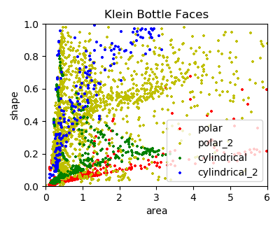
For the polar transform, the basetype was changed to a split geometry since the transform was not identical at θ = 0 and θ = 2π.

klein = s3d.PolarSurface(rez+1,basetype='hex_s',color=color,lw=lw,name='polar_2' )
bottles[1] = klein.map_geom_from_op( polar_klein2, returnxyz=True )

klein = s3d.CylindricalSurface(rez,color=color,lw=lw,name='cylindrical_2' )
bottles[3] = klein.map_geom_from_op( cylin_klein2, returnxyz=True )

This visualization is ‘smoother’ than the example due to the uniform distribution of vertices in the parametric dependent variables. This use of the planar and cylindrical base and split surfaces is often useful for parametric functions for this reason, even though the functions may be expressed in other native coordinates.

Bottom line: One base fits all. However, some bases fit better than others.