Projecting contour profiles

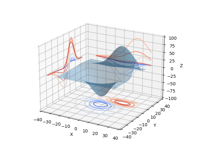
This is a comparison to the Projecting contour profiles onto a graph Matplotlib example. The get_projected_Contours method combines the multiple steps of creating the contour set, color mapping, and projecting the contour onto a plane. This method then has a similar argument list as the Matplotlib axis contour method.

import copy
import numpy as np
import matplotlib.pyplot as plt
from mpl_toolkits.mplot3d import axes3d
import s3dlib.surface as s3d

#.. Matplotlib Examples: Projecting contour profiles onto a graph

# Figure 1 ===============================================================

# 1. Define function to examine .....................................

X, Y, Z = axes3d.get_test_data()

def get_projected_Contours( surface, stride, zdir, offset, cmap) :
    dmap, direction = { 'x':0 , 'y':1, 'z':2 }, [0,0,0]
    direction[ dmap[zdir] ] = 1
    surface = copy.copy(surface)  #.. so original surface coloring is preserved
    surface.map_cmap_from_op( lambda xyz : xyz[dmap[zdir]],cmap)
    contours = surface.contourLineSet(stride,direction=direction)
    #contours.map_cmap_from_op( lambda xyz : xyz[dmap[zdir]],cmap)
    contours.map_to_plane( offset,direction=direction )
    return contours

# 2. Setup and map surfaces .........................................
rez=4

surface = s3d.PlanarSurface(rez, basetype='oct1')
surface.map_geom_from_datagrid( Z ).scale_dataframe(X,Y,Z)
surface.set_surface_alpha(0.3).shade()

x_contours = get_projected_Contours(surface,8,'x', -40,'coolwarm')
y_contours = get_projected_Contours(surface,8,'y',  40,'coolwarm')
z_contours = get_projected_Contours(surface,8,'z',-100,'coolwarm')

# 3. Construct figure, add surface, plot ............................

fig = plt.figure()
ax = plt.axes(projection='3d')
ax.view_init(20)
ax.set(xlim=(-40, 40), ylim=(-40, 40), zlim=(-100, 100),
    xlabel='X', ylabel='Y', zlabel='Z')

ax.add_collection3d(surface)
ax.add_collection3d(x_contours)
ax.add_collection3d(y_contours)
ax.add_collection3d(z_contours)

The separation of each of the three operational steps provides additional flexibility for creating visualizations. The Contour Projections and Complex Cylindrical Contours examples use the line color derived from the surface coloring. The Colored Surface Contour Set contours plot is constructed from a plane which is not normal to the coordinate axes. The General Surface Contour Projections example uses three different direction vectors for planar contour normals, colormapping direction and contour planar projection.

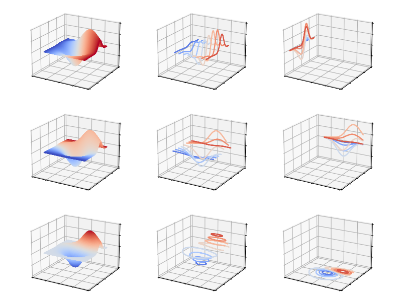
The following figure shows each step. Each row shows the steps for the x, y, and z projected contours.

fig.tight_layout(pad=1)

# Figure 2 ===============================================================

rez,stride,off = 6, 8, [-40,40,-100]

fig = plt.figure(figsize=[8,6])
for dcoor in range(0,3) :
    direction = [0,0,0]
    direction[dcoor]=1
    # 1. create surface
    surface = s3d.PlanarSurface(rez, basetype='oct1')
    surface.map_geom_from_datagrid( Z ).scale_dataframe(X,Y,Z)
    surface.map_cmap_from_op(lambda c:c[dcoor],'coolwarm')
    # 2. create contours
    contours = surface.contourLineSet(stride,direction=direction)
    # 3. project contours
    proj_cont = copy.copy(contours) # so unprojected contour object is preserved
    proj_cont.map_to_plane( off[dcoor],direction=direction )

    obj = [surface,contours,proj_cont]
    for vobj in range(0,3) :
        i = 3*dcoor + vobj
        ax = fig.add_subplot(3,3,i+1, projection='3d')
        ax.view_init(20)
        ax.set(xlim=(-40, 40), ylim=(-40, 40), zlim=(-100, 100) )
        ax.tick_params(labelcolor='w')